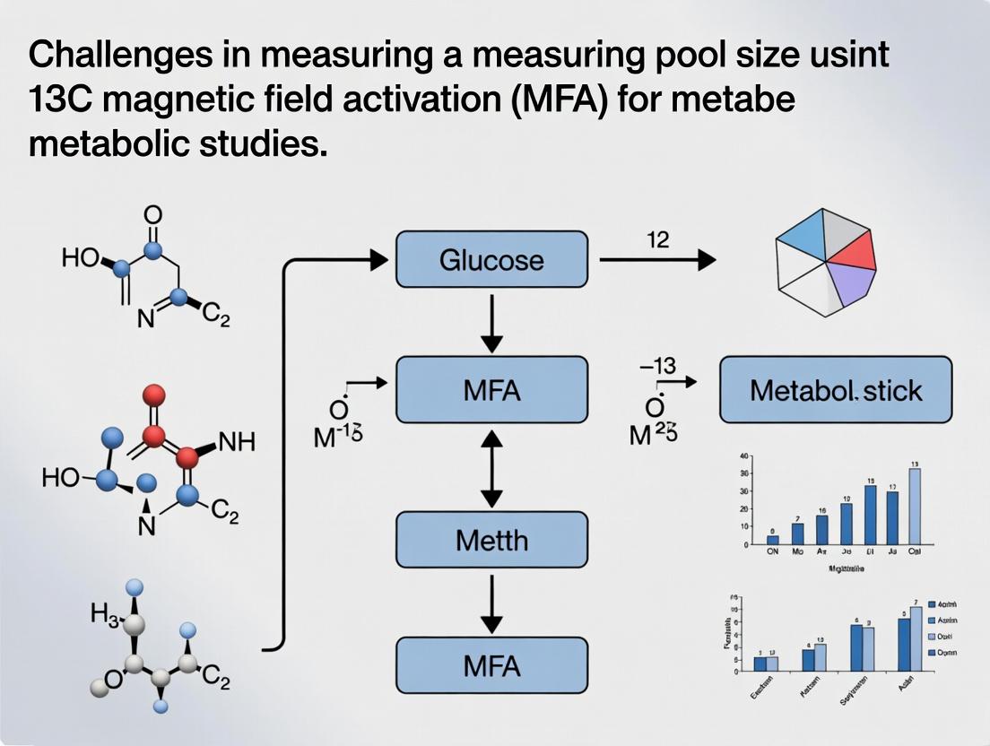
Navigating 13C MFA Metabolite Pool Size Challenges: A Guide for Systems Biology & Drug Discovery Researchers
This article provides a comprehensive analysis of the technical and analytical challenges in measuring intracellular metabolite pool sizes for 13C Metabolic Flux Analysis (MFA).
Navigating 13C MFA Metabolite Pool Size Challenges: A Guide for Systems Biology & Drug Discovery Researchers
Abstract
This article provides a comprehensive analysis of the technical and analytical challenges in measuring intracellular metabolite pool sizes for 13C Metabolic Flux Analysis (MFA). Targeted at researchers and drug development professionals, it covers foundational concepts, methodological best practices, common troubleshooting strategies, and validation protocols. By addressing isotopic dilution, quenching artifacts, analytical sensitivity, and model integration, the article offers a roadmap to obtain more accurate and physiologically relevant flux maps, crucial for advancing metabolic research in biomedicine and therapeutic development.
Why Pool Size Matters in 13C MFA: Defining the Problem and Its Impact on Flux Accuracy
The Critical Role of Intracellular Metabolite Concentrations in Constraint-Based Flux Models
Technical Support Center: Troubleshooting 13C MFA & Pool Size Integration
Frequently Asked Questions (FAQs)
Q1: Our constraint-based flux model, after integrating quantitative metabolomics data, shows physiologically impossible flux loops (futile cycles). What is the most likely cause and how can we resolve it? A1: This often stems from incorrect assignment of metabolite compartmentalization or assuming homogeneity where distinct subcellular pools exist. The model may be satisfying constraints by creating artificial cycles between mis-assigned pools.
- Troubleshooting Protocol:
- Verify Compartmentalization: Re-examine your literature and database evidence (e.g., UniProt, Arabidopsis Subcellular Database) for each metabolite's known localization.
- Implement Pool Splitting: In your model (e.g., COBRApy script), split the ambiguous metabolite into distinct compartmentalized versions (e.g.,
glc_candglc_m). - Add Transport Reactions: Introduce explicit, often reversible, transport reactions between the new compartments with realistic kinetics if available.
- Re-constrain with Data: Apply the measured concentration data to the correct compartmentalized pool and re-run the simulation (e.g., pFBA, MC sampling). This typically eliminates non-physiological loops.
Q2: When we incorporate our LC-MS/MS measured absolute metabolite concentrations as constraints, the model becomes infeasible. What are the primary checkpoints? A2: Infeasibility indicates a conflict between the stoichiometric constraints, the flux bounds, and the new concentration constraints. Follow this diagnostic tree.
- Diagnostic Workflow:
- Check Unit Consistency: Ensure your concentration units (µmol/gDW) are compatible with your model's flux units (typically mmol/gDW/hr). Inconsistent units by a factor of 1000 are a common error.
- Review Thermodynamics: Use a tool like
eQuilibratorto check if the measured metabolite concentrations, when combined with estimated flux ranges, violate reaction Gibbs free energy (ΔG) constraints. An impossible ΔG will break feasibility. - Relax and Identify: Temporarily relax the concentration bounds by 1-2 orders of magnitude. Systematically tighten them back while tracking which constraint(s) cause infeasibility. This identifies the "culprit" metabolite(s) whose measurements may be outliers or require re-examination of their associated network topology.
Q3: For precise pool size measurement in 13C MFA, what is the optimal sampling protocol to capture rapid turnover in central carbon metabolism? A3: Traditional quenching in cold methanol can lead to leakage and underestimation of labile pools, skewing integrated models.
- Optimized Rapid Sampling Protocol:
- Equipment: Use a fast-quenching device (e.g., a automated syringe plunge into -40°C 60% aqueous methanol with dry ice bath, or a dedicated rapid sampling instrument).
- Timing: For microbes, take samples at 5, 15, 30, 45, 60, and 90 seconds after perturbation/label introduction. For mammalian cells, initial points may be at 15, 30, 60, 120 seconds.
- Processing: Immediately vortex, transfer to -80°C, then lyophilize. Reconstitute in MS-compatible solvent.
- Internal Standards: Add isotopically labeled internal standards at the quenching step to correct for any losses during processing.
Q4: How do we handle discrepancies between enzyme saturation levels inferred from measured metabolite concentrations (e.g., via KM values) and fluxes predicted by the model? A4: This discrepancy is a key insight, often pointing to allosteric regulation or incorrect enzyme kinetic parameters.
- Resolution Guide:
- Calculate Saturation: For a metabolite M and enzyme E, compute [M] / (Km + [M]). A low value (<0.5) suggests the enzyme is not saturated.
- Compare to Flux Control: If the model predicts a high flux through E but the saturation is low, investigate:
- Allosteric Activators: Check literature for positive regulators (e.g., ADP for PFK1) whose in vivo concentration may be high.
- Post-Translational Modification: The enzyme activity may be modulated by phosphorylation etc., not reflected in the in vitro Km.
- Parameter Uncertainty: The in vitro Km may not reflect the in vivo condition. Consider using the concentration data to perform Monte Carlo sampling within uncertainty ranges of Km to see if fluxes can be reconciled.
Table 1: Typical Intracellular Metabolite Concentrations in E. coli (Central Carbon Metabolism)
| Metabolite | Compartment | Typical Range (mM) | Notes for Model Constraining |
|---|---|---|---|
| Glucose-6-Phosphate | Cytosol | 2.1 - 4.8 | Key branch point. Constrain upper bound to reflect feedback inhibition on hexokinase. |
| ATP | Cytosol | 1.5 - 3.5 | Use [ATP]/[ADP] ratio (∼10) as a thermodynamic constraint for energy-consuming reactions. |
| NADH | Cytosol | 0.1 - 0.4 | Use [NADH]/[NAD+] ratio as a constraint on oxidative reactions. Highly compartment-specific. |
| Acetyl-CoA | Cytosol | 0.05 - 0.2 | Very low, thermodynamically drives TCA cycle and fatty acid synthesis. |
| 2-Oxoglutarate | Mitochondrial | 0.05 - 0.15 | Critical: Distinct from cytosolic pool. Incorrect pooling invalidates TCA/ANAplerotic flux estimates. |
| Glycine | Mitochondrial | 1.5 - 5.0 | Important for one-carbon metabolism. Compartmentation is essential for cancer metabolism models. |
Table 2: Impact of Pool Size Constraints on Flux Prediction Uncertainty (Monte Carlo Simulation)
| Model Scenario | Glucose Uptake Flux CV (%) | TCA Cycle Flux (Succinate Dehydrogenase) CV (%) | Pentose Phosphate Pathway Flux CV (%) |
|---|---|---|---|
| Unconstrained Metabolite Pools | 22.5 | 45.7 | 68.3 |
| Constrained by Relative (GC-MS) Data | 18.1 | 32.4 | 41.9 |
| Constrained by Absolute (LC-MS/MS) Pool Sizes | 9.8 | 15.2 | 18.5 |
| Constrained by Pools + Thermodynamics (ΔG) | 6.3 | 11.1 | 13.7 |
Experimental Protocols
Protocol 1: Integrated 13C-MFA with Absolute Quantitation for Constraint-Based Modeling Objective: To generate mutually consistent datasets of metabolic fluxes and absolute intracellular metabolite concentrations for genome-scale model refinement.
- Cell Cultivation & Labeling: Grow cells in a controlled bioreactor. At mid-exponential phase, switch to a feed containing a 13C-labeled carbon source (e.g., [1,2-13C]glucose) using a rapid medium switcher.
- Dual Quenching & Sampling:
- For Fluxomics: At steady-state labeling (determined empirically), rapidly sample and quench 5-10 ml culture in -40°C 60% methanol. Pellet, wash, store at -80°C for later GC-MS analysis of proteinogenic amino acids.
- For Absolute Metabolomics: In parallel, rapidly filter 2-5 ml culture on a vacuum filtration manifold (0.45µm nylon filter), immediately plunge the filter into 3 ml of -20°C 80% acetonitrile/water with internal standards. Sonicate on ice, centrifuge, and dry supernatant for LC-MS/MS.
- Mass Spectrometry Analysis:
- Flux (GC-MS): Derivatize protein hydrolysate with MTBSTFA. Analyze on GC-MS. Fit labeling patterns to model using software like INCA or Isotopomer Network Compartmental Analysis.
- Concentration (LC-MS/MS): Reconstitute in H2O. Use HILIC chromatography coupled to a triple-quadrupole MS in MRM mode. Quantify against a standard curve of unlabeled analytes, normalized to cell dry weight.
- Data Integration: Convert absolute concentrations (µmol/gDW) to mM using published cellular volume data. Apply these as additional inequality constraints (
lb < concentration < ub) in the stoichiometric matrix (S) of your constraint-based model (e.g., in CobraPy). Perform flux variability analysis (FVA) to assess solution space reduction.
Protocol 2: Validating Model Feasibility with Thermodynamic Constraints Objective: Ensure flux distributions are thermodynamically feasible given measured metabolite concentrations.
- Calculate Reaction Gibbs Free Energy (ΔG): For each reaction
iin your network, calculate the standard Gibbs free energy (ΔG°') using eQuilibrator API (equilibrator-api). - Compute in vivo ΔG: Use the formula ΔGi = ΔG°'i + R T ln(Qi), where the reaction quotient Qi is calculated from your measured in vivo metabolite concentrations.
- Apply Directionality Constraints: For reactions where the calculated ΔGi is large and negative (e.g., < -5 kJ/mol), constrain the lower flux bound to be ≥ 0 (irreversible forward). If large and positive, constrain the upper bound to be ≤ 0.
- Run Thermodynamically Constrained FBA (tcFBA): Incorporate these directionality constraints into the model. Re-optimize. The resulting flux distribution will be thermodynamically feasible, resolving many futile cycles.
The Scientist's Toolkit: Research Reagent Solutions
| Item | Function in 13C MFA/Pool Size Research |
|---|---|
| U-13C6 Glucose (or other labeled substrates) | The isotopic tracer that enables quantification of metabolic pathway fluxes through labeling patterns. |
| SILAC-grade Amino Acid Mixtures (13C,15N) | For mammalian cell MFA; provides comprehensive labeling of proteinogenic amino acids for flux determination. |
| Deuterated or 13C-labeled Internal Standards (e.g., d27-Myristic Acid, 13C5-Glutamine) | Added at quenching for absolute metabolomics; corrects for ion suppression and recovery losses during sample prep. |
| Cold Methanol/Acetonitrile (-40°C) | Standard quenching agents to instantaneously halt metabolism. Acetonitrile is preferred for some metabolite classes. |
| Filter Manifold with Nylon Membranes (0.45µm) | Enables rapid separation of cells from medium for metabolomics, much faster than centrifugation. |
| Derivatization Reagent (e.g., MTBSTFA for GC-MS) | Volatilizes polar metabolites (amino acids, organic acids) for analysis by gas chromatography. |
| QC Reference Metabolite Extract (e.g., NIST SRM 1950) | A standardized human plasma sample used to calibrate and ensure inter-laboratory reproducibility in LC-MS/MS. |
Visualization Diagrams
Diagram 1: Model Infeasibility Diagnostic Tree
Diagram 2: Integrated 13C MFA & Metabolomics Workflow
Technical Support Center
Troubleshooting Guides & FAQs
Q1: Why do my measured intracellular metabolite pool sizes show high variance despite using the isotopic dilution method? A: High variance often stems from inconsistent quenching and extraction. The rapid turnover of central carbon metabolites requires quenching to occur in <1 second. Ensure your quenching solution (e.g., 60% methanol at -40°C) is of sufficient volume and is rapidly mixed. Validate extraction efficiency by spiking with known amounts of unlabeled standard compounds prior to cell lysis and comparing LC-MS peak areas.
Q2: During non-stationary 13C labeling (INST-MFA), my label incorporation data does not fit any model. What are the primary culprits? A: This is typically due to incorrect assumptions about the labeling input or metabolic steady-state prior to perturbation.
- Verify the labeling purity of your tracer (e.g., [U-13C6]glucose). Degradation or contamination can alter the initial labeling state.
- Confirm metabolic steady-state before the pulse. Measure extracellular rates (uptake/secretion) for at least 3 cell residence times to ensure stability.
- Check sampling timepoints. Early timepoints (5-15 seconds) are critical for flux estimation. Use a rapid sampling setup (e.g., automated quenching module).
Q3: How do I distinguish between true isotopic dilution from natural abundance and dilution from unlabeled carbon sources in the media? A: You must run a control experiment using a naturally abundant (unlabeled) carbon source under identical conditions. The mass isotopomer distribution (MID) from this control represents the background from natural 13C abundance and any unlabeled media components. Subtract this background MID vector from your experimental MID before calculating pool sizes or fitting fluxes.
Q4: My GC-MS fragments cause overlapping isotopomer distributions, confounding pool size estimation. How can I resolve this? A: Use LC-MS/MS if possible for better separation. If using GC-MS, you must apply a correction matrix. Derive the matrix by analyzing pure standards of the metabolite to determine the fractional contribution of each carbon position to each detected mass fragment (m/z). Apply this matrix mathematically to deconvolve the measured MIDs.
Q5: What is the impact of compartmentation (e.g., cytosolic vs. mitochondrial pools) on pool size measurements? A: Compartmentation is a major challenge. If a metabolite exists in distinct, non-mixing pools, the measured pool size is an aggregate and the MID is a weighted average. This can severely bias flux estimates. Strategy: Use enzymatic assays or fractionation to isolate compartments, or refine your metabolic network model to include separate pools for key metabolites like acetyl-CoA or glutamate.
Experimental Protocols
Protocol 1: Rapid Sampling for INST-MFA Metabolite Quenching and Extraction
- Culture Preparation: Grow cells in a controlled bioreactor to steady-state (constant cell density, substrate, and product concentrations).
- Tracer Pulse: Rapidly switch the feed medium to an identical medium containing the 13C tracer (e.g., swap from 100% natural glucose to 100% [1-13C]glucose). Use a fast-responding system.
- Rapid Sampling: At predetermined timepoints (e.g., 5, 10, 15, 30, 60, 120 seconds), withdraw a known volume of culture (1-2 mL) and immediately inject it into 5-10 volumes of pre-chilled (-40°C) quenching solution (60% aqueous methanol) with vigorous vortexing.
- Metabolite Extraction: Pellet cells at -20°C. Resuspend pellet in cold extraction solvent (e.g., 40:40:20 methanol:acetonitrile:water with 0.5% formic acid). Sonicate on ice for 5 minutes.
- Analysis: Centrifuge, collect supernatant, dry under nitrogen, and reconstitute in MS-compatible solvent for LC-MS analysis.
Protocol 2: Absolute Quantification for Pool Size via Isotopic Dilution
- Internal Standard Spike: Immediately after quenching, add a known quantity (e.g., 10 pmol) of a uniformly 13C-labeled (U-13C) version of the target metabolite as an internal standard. This standard has a known MID.
- Co-extraction: Proceed with standard extraction (as in Protocol 1, step 4). The U-13C standard undergoes identical losses.
- LC-MS/MS Analysis: Use a Multiple Reaction Monitoring (MRM) transition specific to the metabolite. Quantify the natural (unlabeled) metabolite peak area (M+0) relative to the peak area of the fully labeled standard (e.g., M+n for an n-carbon molecule).
- Calculation: Pool size = (AreaM0sample / AreaM+nstandard) * Amount of U-13C standard added.
Data Presentation
Table 1: Common Tracers and Their Application in 13C MFA Pool Size Studies
| Tracer Compound | Labeling Pattern | Primary Metabolic Pathways Probed | Key Challenges for Pool Size |
|---|---|---|---|
| Glucose | [1-13C] | PPP, Glycolysis, TCA Anaplerosis | Recycling via gluconeogenesis dilutes label. |
| Glucose | [U-13C6] | Complete network mapping, parallel pathways | Cost; may require correction for natural abundance. |
| Glutamine | [U-13C5] | TCA cycle, reductive metabolism, nucleotide synthesis | Rapid equilibration with glutamate pool. |
| Acetate | [1,2-13C2] | Acetyl-CoA metabolism, lipogenesis | Low uptake rates in some cell lines. |
| NaHCO3 | [13C] | Anaplerotic fluxes (pyruvate carboxylase) | Requires tightly sealed culture system to prevent loss. |
Table 2: Comparison of Metabolite Extraction Solvents for INST-MFA
| Solvent System (MeOH:ACN:H2O) | Acid/Base Additive | Extraction Efficiency (Relative) | Suitability for INST-MFA | Key Drawback |
|---|---|---|---|---|
| 40:40:20 | 0.5% Formic Acid | High (Broad Range) | Excellent for polar, acidic metabolites | May hydrolyze labile metabolites. |
| 40:40:20 | 0.5% Ammonium Hydroxide | High (Basic Metabolites) | Good for nucleotides, CoA species | Not suitable for organic acids. |
| 60:20:20 | None | Moderate | Simple, no additive interference | Lower efficiency for charged metabolites. |
| 80:20 (MeOH:H2O) | None | High (Polar Metabolites) | Fast, common for quenching/extraction | May precipitate hydrophobic compounds. |
Visualizations
Title: Non-Stationary 13C Labeling Experimental Workflow
Title: Compartmentation Challenge & Solutions in 13C MFA
The Scientist's Toolkit: Research Reagent Solutions
| Item | Function & Importance |
|---|---|
| Fully 13C-Labeled (U-13C) Internal Standards | Crucial for absolute quantification via isotopic dilution. Added post-quenching to correct for extraction losses. |
| Quenching Solution (60% Methanol, -40°C) | Instantly halts metabolism. Must be cold and in large volume relative to culture to ensure rapid temperature drop. |
| Dual-Phase Extraction Solvent (e.g., Methanol/Chloroform/Water) | Used for lipidomic studies alongside metabolomics, partitioning metabolites and lipids into separate phases. |
| Stable Isotope Tracers (e.g., [U-13C6]Glucose) | The perturbation agent. Purity (>99% 13C) is critical. Must be sterile-filtered for bioreactor use. |
| Rapid Sampling Device (e.g., Syringe + Pre-filled Quench Tube) | Enables manual sampling at sub-5-second intervals for early INST-MFA timepoints. |
| Automated Sampling/Robo-Platform | For high-temporal-resolution sampling (multiple sub-second points), removing manual variability. |
| LC-MS Column (HILIC, e.g., BEH Amide) | Separates polar, non-derivatized central carbon metabolites for accurate MID measurement. |
| Flux Estimation Software (e.g., INCA, 13CFLUX2) | Integrates INST-MFA data, network model, and pool sizes to compute fluxes via iterative fitting. |
Troubleshooting Guide & FAQs
Q1: My 13C MFA data shows poor fit for specific metabolite pool sizes. Is this more likely due to biological variation or a technical issue with my extraction protocol? A1: This is a common challenge. First, systematically check your technical pipeline. Ensure your quenching and extraction protocol is optimized for your specific cell type—rapid cooling is critical to halt metabolism instantly. A common technical error is incomplete cell disruption leading to underestimation of pool sizes. Run a spike-in recovery experiment using a known amount of an unlabeled standard not native to your system (e.g., norvaline for amino acids) during extraction to quantify technical losses. If recovery is >90%, the variability is likely biological. Biological replicates (n≥5) are then essential to quantify inter-culture variation.
Q2: How can I distinguish between variability introduced by the MS instrument versus biological replication? A2: Implement a rigorous experimental design with Quality Control (QC) samples. Prepare a large, homogeneous pool of extracted sample from one culture. Inject this QC sample at least 3-5 times throughout your MS run sequence. The variance in pool size estimates from these repeated injections quantifies technical variability (instrument + data processing). The variance between independently cultured and processed samples quantifies total variability. Biological variability is estimated as: σ²biological = σ²total - σ²_technical.
Q3: My isotopic labeling patterns are inconsistent between replicates. What are the primary sources of this variability? A3: Inconsistent labeling often points to upstream biological or experimental variability. Key sources include:
- Biological: Minor differences in cell physiology at harvest (e.g., slight variations in confluence, nutrient depletion, or dissolved O₂).
- Technical: Inaccurate timing of the labeling pulse, incomplete mixing of the labeled tracer in the bioreactor, or delays during quenching. Ensure the labeling medium is pre-warmed and added swiftly and evenly.
Q4: What are the best practices for error propagation in 13C MFA to account for both biological and technical variance in pool size estimates? A4: Do not rely solely on the model-fitting residuals. Use a Monte Carlo simulation approach:
- Quantify the measurement error (technical variance) for each mass isotopomer from your QC sample data.
- For each biological replicate, generate hundreds of simulated datasets by perturbing the raw mass spectrometry data within the bounds of the measured technical error.
- Fit the model to each simulated dataset.
- The distribution of resulting pool size estimates captures the propagated technical uncertainty. The spread of best-fit estimates from the true biological replicates then provides the biological uncertainty.
Essential Experimental Protocols
Protocol 1: Spike-in Recovery Experiment for Extraction Efficiency
- Preparation: Prepare a stock solution of your non-native standard (e.g., 2mM norvaline in 50% methanol).
- Spike-in: At the moment of cell extraction, add a precise volume of this stock directly to the extraction solvent/cell mixture immediately upon contact.
- Processing: Complete the extraction protocol as usual.
- Analysis: Quantify the recovered amount of the spike-in standard via LC-MS/MS against a calibration curve. Compare to the amount added.
- Calculation: % Recovery = (Measured concentration / Expected concentration) * 100.
Protocol 2: Sequential QC Sample Injection for Technical Variance Estimation
- QC Pool Creation: Grow a large culture, quench, and extract cells following your standard protocol. Pool all extracts into a single, homogenous vial. Aliquot and store at -80°C.
- Run Sequence Design: For a batch of n biological samples, create an injection sequence: Blank → QC → Sample 1 → Sample 2 → QC → Sample 3 → ... → Sample n → QC.
- Data Analysis: Extract the peak areas/intensities for your metabolites of interest from each QC injection. Calculate the Coefficient of Variation (CV = standard deviation/mean) for each analyte across the QCs. A CV > 15% typically indicates significant instrument-derived technical noise for that analyte.
Table 1: Typical Sources of Variability in 13C MFA Pool Size Estimation
| Variability Type | Source Category | Examples | Impact on Pool Size Estimate |
|---|---|---|---|
| Biological | Physiological State | Cell cycle distribution, metabolic heterogeneity in population | Fundamental limit to precision; reflects true biological diversity. |
| Biological | Culture Conditions | Micro-environmental differences in bioreactor (pH, O₂, nutrients) | Can be minimized by stringent process control. |
| Technical | Sample Preparation | Quenching speed, extraction efficiency, metabolite degradation | Causes systematic bias (under/overestimation). |
| Technical | Instrumentation | MS detector drift, injection volume inaccuracy, column performance | Contributes to random error across runs. |
| Technical | Data Processing | Peak integration boundaries, noise filtering, background subtraction | Affects accuracy of isotopic labeling patterns. |
Table 2: Quantitative Comparison of Variability from a Representative 13C MFA Study (Simulated Data)
| Metabolite Pool | Mean Size (μmol/gDW) | Biological CV (%) (n=6) | Technical CV (%) (QC, n=5) | Total Observed CV (%) |
|---|---|---|---|---|
| Glucose-6-Phosphate | 1.25 | 18.2 | 6.1 | 19.2 |
| 3-Phosphoglycerate | 0.42 | 22.5 | 8.7 | 24.1 |
| Pyruvate | 0.85 | 14.8 | 12.3 | 19.3 |
| Lactate | 5.60 | 9.5 | 4.2 | 10.4 |
| ATP | 3.10 | 7.1 | 5.5 | 9.0 |
CV: Coefficient of Variation; gDW: gram Dry Weight. Technical CV derived from repeated injection of a pooled extract.
Visualizations
Title: Sources of Uncertainty in Pool Size Estimates
Title: 13C MFA Workflow with Key QC Steps
The Scientist's Toolkit: Research Reagent Solutions
| Item | Function & Importance in Reducing Variability |
|---|---|
| [-40°C, 40:40:20 Methanol:Acetonitrile:Water + Buffers] | Cold Quenching Solution: Rapidly cools cells and halts enzyme activity. Consistent temperature and composition are critical for reproducible quenching. |
| Internal Standard Spike-in Kit (e.g., 13C/15N-labeled cell extract or non-native standards) | Extraction & Instrument Control: Corrects for losses during sample preparation and matrix effects during MS analysis, reducing technical variance. |
| Stable Isotope Tracer (e.g., [U-13C]Glucose, [1,2-13C]Glucose) | MFA Substrate: High isotopic purity (>99%) is essential to avoid errors in labeling pattern measurement and model fitting. |
| Derivatization Reagents (e.g., MCF for GC-MS) | Volatilization for GC: Converts polar metabolites to volatile derivatives. Fresh, high-purity reagents prevent side reactions that introduce technical noise. |
| Retention Time Index Standards (for LC-MS) | Chromatographic Alignment: Allows correction for minor drift in retention time across long sequences, improving peak alignment accuracy. |
| Quality Control Pooled Extract | System Suitability Monitor: A homogenous sample used to track instrument performance over time and quantify technical precision. |
Troubleshooting Guides & FAQs for 13C MFA Pool Size Measurements
Q1: During a 13C MFA experiment, my calculated flux distribution is highly sensitive to small changes in the measured labeling pattern of a specific central carbon intermediate (e.g., PEP). What could be the cause and how can I resolve it? A: This often indicates an incorrectly assumed or poorly constrained intracellular pool size for that metabolite. The pool size directly impacts the apparent labeling kinetics. To resolve:
- Validate Quenching & Extraction: Ensure your quenching method (e.g., cold methanol/water at -40°C) instantly halts metabolism. Incomplete quenching leads to pool size artifacts.
- Implement Direct Pool Size Measurement: Use an LC-MS/MS protocol with external calibration curves using authentic standards, in parallel with your 13C labeling experiment. Use an internal standard (e.g., 13C/15N-labeled cell extract) for absolute quantification.
- Perform Time-Course Labeling: Conduct the 13C tracer experiment over multiple, closely spaced time points (e.g., 0, 15, 30, 60, 120 seconds). Fit both fluxes and pool sizes simultaneously using computational software (INCA, OMIX) to identify the combination that best explains the dynamics of labeling.
Q2: I observe rapid 13C labeling in ATP but very slow labeling in NADH, complicating my flux analysis. How should I interpret this and adjust my model? A: This is expected due to different pool sizes and turnover rates. ATP is a large, rapidly turning over "energy currency" pool. NADH is smaller and its labeling is compartmentalized (cytosol vs. mitochondria).
- Action: Do not assume a single, homogeneous pool for cofactors. For eukaryotic cells, model cytosolic and mitochondrial NADH/NAD+ pools separately in your MFA model. Use enzyme activity data or literature to constrain the transfer between compartments. The rapid ATP labeling can be used as a sanity check for your estimated energy metabolism fluxes.
Q3: My LC-MS data for central metabolites (like G6P, 3PG) shows high technical variance, making pool size estimation unreliable. What are the key steps to improve reproducibility? A: High variance typically stems from sample preparation, not the instrument.
- Protocol Fix:
- Cell Counting: Precisely normalize biomass before quenching (per cell count, not just culture volume).
- Quenching: Add quenching solution (60% cold aqueous methanol, -40°C) directly and rapidly to culture with vigorous mixing. Maintain <-20°C throughout.
- Extraction: Use a biphasic chloroform/methanol/water extraction for comprehensive polar metabolite recovery. Include a bead-beating step for microbial cells.
- Internal Standards: Spike a uniform 13C-labeled cell extract (commercially available for E. coli/yeast) or a cocktail of chemically similar, stable isotope-labeled standards (e.g., 13C6-G6P, D7-ATP) at the very beginning of extraction to correct for losses.
Q4: When attempting to measure ATP/ADP/AMP ratios alongside 13C labeling, the ratios appear artificially shifted towards low energy charge. How can I preserve the in-vivo state? A: You are likely observing enzymatic degradation during sample processing. ATP is labile.
- Solution: Modify your extraction protocol to include strong, instant acid denaturation. For example, after cold methanol quenching, resuspend the pellet in 0.5M perchloric acid or 1M formic acid (containing known amounts of 13C10-ATP as an internal standard). Immediately neutralize with KOH/KHCO3 after 30 seconds on ice. Pellet the potassium perchlorate salt and use the supernatant for LC-MS.
Research Reagent Solutions Toolkit
| Item | Function in 13C MFA Pool Size Analysis |
|---|---|
| U-13C6 Glucose | The most common tracer for mapping central carbon metabolism (glycolysis, PPP, TCA). |
| Uniformly 13C-labeled Cell Extract (e.g., from E. coli) | Served as a comprehensive internal standard for absolute quantification of pool sizes and correction for matrix effects in MS. |
| Stable Isotope-Labeled Internal Standards (e.g., 13C10-ATP, 15N5-ATP, D7-NADH) | Chemical analogues spiked at quenching for specific, accurate quantification of labile cofactor pools. |
| Cold Methanol/Water (60:40, v/v) at -40°C | Standard quenching solution to instantly freeze metabolism. |
| Biphasic Chloroform/Methanol/Water Extraction Solvents | Provides high recovery for both polar metabolites (aqueous phase) and lipids (organic phase). |
| Reconstitution Buffer (e.g., 10 mM NH4Ac in water, pH 9) | Optimal LC-MS mobile phase for hydrophilic interaction (HILIC) chromatography of central metabolites. |
| HILIC Chromatography Column (e.g., BEH Amide) | Separates polar, isomeric metabolites (e.g., G6P/F6P) prior to MS detection. |
| High-Resolution Mass Spectrometer (Q-TOF or Orbitrap) | Resolves 13C isotopic fine structure (isotopologue distributions) essential for MFA. |
Table 1: Approximate Intracellular Concentrations in E. coli (from literature)
| Metabolite Pool | Estimated Concentration (mM) | Notes / Variability |
|---|---|---|
| ATP | 3 - 10 | Varies strongly with growth rate and energy charge. |
| ADP | 0.5 - 2 | |
| AMP | 0.1 - 0.5 | |
| NADH | 0.1 - 0.3 | Much lower than NAD+; mitochondrial pool is distinct. |
| NAD+ | 2 - 4 | |
| Glucose-6-Phosphate | 1 - 3 | Sensitive to glycolytic flux. |
| Phosphoenolpyruvate | 0.5 - 2 | Key node connecting glycolysis to TCA/anapleurosis. |
| Acetyl-CoA | 1 - 5 | Cytosolic and mitochondrial pools differ significantly. |
Detailed Experimental Protocol: Simultaneous Metabolite Pool Size and 13C Labeling Measurement
Title: Integrated Sampling for 13C MFA and Absolute Quantitation
Workflow:
- Culture & Labeling: Grow cells in bioreactor or controlled chemostat. Switch medium to one containing the desired 13C tracer (e.g., U-13C Glucose) rapidly. Use a fast-filtration manifold or rapid-sampling setup.
- Quenching: At defined time points (0, 15s, 30s, 1, 2, 5, 10 min), draw 5-10 mL of culture and immediately vacuum-filter onto a pre-chilled (-40°C) nylon membrane. Immediately wash with 10 mL of 60% cold aqueous methanol.
- Extraction: Transfer filter with biomass to 2 mL tube with 1 mL of -20°C extraction solvent (40:40:20 Methanol:Acetonitrile:Water with 0.5% Formic Acid) containing your spiked internal standards. Agitate vigorously (bead-beat) for 3 minutes at 4°C.
- Processing: Centrifuge at 16,000 g for 10 min at 4°C. Transfer supernatant to a new tube. Dry under a gentle nitrogen stream.
- LC-MS Analysis: Reconstitute in 100 µL HILIC-compatible buffer. Analyze via HILIC-HRMS.
- MS Method: Full scan (high resolution >60,000) for isotopologue detection. Parallel Reaction Monitoring (PRM) for sensitive quantification of internal standards and low-abundance cofactors.
- Data Processing: Use software (e.g., Maven, El-MAVEN, XCMS) to integrate peak areas for all isotopologues. For absolute quantitation, use the internal standard response ratio against an external calibration curve run in the same batch.
Diagrams
Title: Integrated Workflow for 13C MFA & Pool Quantitation
Title: Cofactor & Metabolite Pool Compartmentalization
Technical Support Center: 13C MFA Pool Size Quantification & Troubleshooting
FAQ & Troubleshooting Guides
Q1: Our 13C-MFA flux solution fits the labeling data well (low SSR), but the predicted pool sizes seem biologically implausible. What could be the cause? A: A good statistical fit with implausible pool sizes often indicates an identifiability issue. The network model may lack the necessary constraints to uniquely determine both fluxes and metabolite concentrations (pool sizes). This is common when using only steady-state labeling data without direct size measurements.
- Troubleshooting Steps:
- Check Network Completeness: Ensure all relevant reversible reactions and parallel pathways (e.g., pentose phosphate vs. glycolysis) are included. Missing reactions can force errors into pool size estimates.
- Perform Sensitivity Analysis: Use your MFA software (e.g., INCA, COBRA) to calculate the sensitivity matrix or confidence intervals for each pool size. Large confidence intervals (>50% of the value) indicate the parameter is poorly identified.
- Incorporate Additional Data: Integrate quantitative metabolomics data (e.g., from LC-MS) as additional constraints in the fitting procedure to anchor pool sizes.
Q2: When we integrate quantitative metabolomics data to constrain pool sizes, the flux fit degrades significantly. How should we proceed? A: This conflict reveals a critical inconsistency, often between snapshot metabolomics (rapid quenching) and averaged 13C labeling (from a longer labeling experiment).
- Troubleshooting Protocol:
- Audit Quenching & Extraction: Validate your metabolomics sample quenching protocol. Incomplete or slow quenching allows metabolism to continue, altering measured concentrations. Perform a time-course quenching test.
- Verify Culture Steady-State: Confirm that both the cell growth (OD, doubling time) and extracellular metabolites are in steady-state for the entire duration of the 13C labeling experiment prior to sampling for metabolomics.
- Systematic Comparison: Use the table below to diagnose mismatches:
| Data Type | What it Represents | Primary Source of Error | Resolution Strategy |
|---|---|---|---|
| 13C Labeling Pattern | Time-averaged flux state over the labeling period. | Instability in growth rate during experiment. | Frequent OD/doubling time measurements. |
| Quantitative Metabolomics | Instantaneous pool size at quenching moment. | Quenching artifact, extraction efficiency variance. | Use internal labeled standards, optimize quenching. |
| Enzyme Activity Assays | Potential capacity, not in vivo activity. | In vitro conditions not reflecting in vivo. | Use as supportive, not absolute, constraints. |
Q3: What are the best experimental practices for obtaining accurate intracellular metabolite pool sizes for constraining MFA models? A: Follow a validated, integrated protocol for coupled 13C-MFA and Absolute Metabolomics.
- Integrated Experimental Protocol:
- Chemostat Cultivation: Establish a carbon-limited chemostat to ensure perfect metabolic and isotopic steady-state. Maintain for >5 residence times before sampling.
- Rapid Sampling & Quenching: Use a dedicated, cold (~-40°C) quenching solution (e.g., 60% methanol with buffer) sprayed directly into the culture via a rapid-sampling device (<1 sec). Immediately submerge in liquid N2.
- Cold Metabolite Extraction: Perform extraction on frozen cell pellets with cold organic solvent (e.g., methanol/acetonitrile/water mix) containing a cocktail of 13C-labeled internal standards for absolute quantification.
- Parallel Samples for MFA: From the same steady-state culture, harvest cells for biomass hydrolysis and GC-MS analysis of proteinogenic amino acids or other polymers for 13C labeling patterns.
- Data Integration: Use a modeling software (e.g., INCA) capable of performing INST-MFA (Isotopically Non-Stationary MFA) or fitting steady-state 13C data with hard/soft constraints on the measured absolute pool sizes.
Visualizations
Diagram Title: Consequences of Inaccurate Pool Sizes
Diagram Title: Integrated Workflow for Accurate MFA
The Scientist's Toolkit: Key Research Reagent Solutions
| Item | Function & Rationale |
|---|---|
| 13C-Labeled Internal Standards (e.g., 13C6- Glucose, 13C5- Glutamine) | Essential for precise quantification of extracellular uptake/secretion rates, a critical input for any flux model. |
| 13C-Cell Extract Internal Standard Mix | A commercially available mix of uniformly 13C-labeled yeast/E. coli cell extract. Used in metabolomics to correct for matrix effects and calculate absolute intracellular concentrations. |
| Quenching Solution: 60% Aqueous Methanol (-40°C) | Rapidly cools and inactivates metabolism. The low temperature and high methanol concentration halt enzyme activity faster than cold saline alone. |
| Extraction Solvent: Methanol/Acetonitrile/Water (40:40:20) | Efficient, cold extraction solvent for a broad range of polar metabolites. Compatible with both LC-MS and GC-MS analysis post-derivatization. |
| Derivatization Reagent (e.g., MSTFA for GC-MS) | Converts non-volatile metabolites (organic acids, sugars) into volatile trimethylsilyl derivatives for 13C labeling analysis via GC-MS. |
| Software: INCA (Isotopomer Network Compartmental Analysis) | Gold-standard software for 13C-MFA capable of integrating labeling data, exchange fluxes, and absolute metabolite pool sizes into a comprehensive model. |
Best Practices for Measuring Metabolite Pool Sizes: From Quenching to Quantification
Technical Support Center
Troubleshooting Guides & FAQs
Q1: Why do my quenched samples show inconsistent metabolite levels between replicates, even with fast sampling? A: Inconsistency often stems from incomplete or uneven quenching. Ensure your quenching solution (e.g., 60% methanol buffered with HEPES or Tris, cooled to -40°C or below) is in a large volume-to-biomass ratio (recommended ≥5:1 v/v) and is rapidly mixed. For microbial cultures, vacuum filtration followed by immediate quenching can improve consistency. Check that the quenching temperature is maintained and that the sample is fully submerged and agitated upon contact.
Q2: How can I prevent the continued enzymatic activity or "leakage" of metabolites from cells during the quenching process itself? A: This is a key artifact in 13C MFA pool size estimation. Use a buffered cold methanol solution, as it better preserves membrane integrity than pure methanol or acetonitrile, reducing leakage. For sensitive cell types (e.g., mammalian cells), consider alternative methods like spraying the culture directly into pre-heated (>70°C) ethanol or a saline solution. Always validate your quenching method by spiking a non-metabolizable labeled standard and checking for its recovery.
Q3: My sampling device (e.g., syringe, automated sampler) is too slow, leading to turnover artifacts. What are the current fastest options? A: For submerged cultures, consider a rapid sampling device with a pneumatic actuator and a direct expulsion valve into cold quenching fluid; these can achieve sampling-to-quench times of <100 ms. For bioreactors, commercial systems like the RapidSampling (Bioengineering AG) or the ROTV (Rapid Quenching Device) can sample and quench within 30-50 ms. For manual setups, pre-filling a syringe with quenching solution before drawing the sample can speed up the process.
Q4: What is the impact of sampling/quenching delay on measured pool sizes for central carbon metabolites like PEP or ATP? A: Metabolites with high turnover rates (e.g., ATP, PEP, fructose-1,6-bisphosphate) are severely affected. A delay of even one second can lead to changes exceeding 50% of the in vivo concentration. This directly compromises 13C MFA by providing inaccurate input for the estimation of flux and pool sizes.
Q5: How do I handle the quenching and extraction of intracellular metabolites from filamentous fungi or tissue samples, which are difficult to penetrate? A: For tough biological matrices, mechanical disruption integrated into the process is key. After rapid sampling into liquid nitrogen (a preferred quencher for some tissues), use a cryogenic ball mill (e.g., Retsch Mixer Mill) to pulverize the frozen material. Then, perform a two-phase extraction with cold methanol/chloroform/water, ensuring the sample remains below -20°C during the initial steps.
Q6: Are there standardized protocols for specific organism types for 13C MFA studies? A: While principles are universal, parameters differ. Below is a comparison of key parameters for common systems.
Table 1: Comparative Parameters for Rapid Quenching Protocols
| Organism Type | Recommended Quenching Solution | Temp. | Sample-to-Quench Time Target | Key Validation Check |
|---|---|---|---|---|
| E. coli / Bacteria | 60% Aq. Methanol with 70 mM HEPES, pH 7.5 | -40°C to -48°C | < 1 second | ATP/ADP ratio stability, absence of cell lysis (OD260) |
| S. cerevisiae | 60% Aq. Methanol (no buffer often used) | -40°C | < 2 seconds | Trehalose as a marker for insufficient quenching |
| Mammalian Cells | 0.9% Saline in 60% Methanol OR Spray into >70°C Ethanol | -40°C / Hot | < 10 seconds (manual) | NAD+/NADH ratio, lactate/pyruvate ratio |
| Plant Tissues | Liquid Nitrogen (LN₂) Immersion | -196°C | As fast as possible | Visual inspection for ice crystal formation avoidance |
| Filamentous Fungi | LN₂ or Cold 100% Methanol (-80°C) | -80°C / -196°C | < 5 seconds | Subsequent efficient powderization in cryo-mill |
Detailed Experimental Protocols
Protocol 1: Rapid Sampling and Cold Methanol Quenching for Microbial Suspension Cultures (E. coli) Objective: To instantaneously halt metabolism for accurate intracellular metabolite measurement. Materials: Rapid sampling device, vacuum flask, quenching solution (-48°C), 0.45 µm nylon membrane filters, forceps. Procedure:
- Pre-cool quenching solution in a dry ice/ethanol bath. Keep forceps in the bath.
- Set up a vacuum filtration manifold. Pre-wet a filter with room-temperature PBS.
- Using the rapid sampler, expel a known volume of culture (e.g., 5 mL) directly onto the center of the filter under vacuum (approx. 15 inHg). Record exact time.
- Immediately (<1 s) after liquid passes through, release vacuum. Use pre-cooled forceps to transfer the filter into 10 mL of cold quenching solution.
- Vortex vigorously for 10 seconds. Store at -80°C until extraction.
- For extraction, thaw on ice, add internal standards, and use a cold methanol/chloroform/buffer extraction.
Protocol 2: LN₂ Quenching and Cryogenic Grinding for Fungal Mycelia Objective: To quench metabolism and physically disrupt tough cell walls for metabolite extraction. Materials: Liquid N₂ dewar, precooled metal spoons or sampler, cryogenic grinding jars and balls, ball mill. Procedure:
- Pre-cool a metal sampling spoon by immersing in LN₂.
- Rapidly scoop mycelial biomass from a surface culture or filter a pellet from liquid culture.
- Plunge the sample immediately into a 50 mL tube filled with LN₂. Submerge for >30 s.
- Transfer the frozen "biscuit" to a pre-cooled grinding jar containing a grinding ball.
- Secure the jar in a cryogenic ball mill and grind at 25 Hz for 2 minutes.
- While still cold, quickly weigh the powder and transfer it to cold extraction solvent.
The Scientist's Toolkit: Research Reagent Solutions
Table 2: Essential Materials for Rapid Sampling & Quenching
| Item/Reagent | Function & Brief Explanation |
|---|---|
| Buffered Cold Methanol Quench Solution | Standard quenching fluid; cold temperature halts enzymes, methanol denatures them, buffer prevents acid-induced hydrolysis. |
| Liquid Nitrogen (LN₂) | Ultimate cryo-quencher; virtually instantaneous freezing, ideal for tissues and tough cells. |
| 0.45 µm Nylon/PVDF Membrane Filters | For rapid vacuum filtration of microbial cells; minimal metabolite binding. |
| Cryogenic Ball Mill (e.g., Retsch MM 400) | Mechanically disrupts frozen biomass into fine powder for uniform and efficient extraction. |
| Automated Rapid Sampling Device (e.g., Bioengineering AG's system) | Provides reproducible sub-second sampling and quenching, eliminating manual delay artifacts. |
| Pre-cooled Metal Sampling Tools (Spoons, Clamps) | Allows immediate transfer of solid/semi-solid samples into LN₂ without thawing. |
| Labeled Internal Standards (e.g., 13C- or 2H- labeled amino acids, sugars) | Spiked into quenching/extraction solution to correct for losses during processing. |
| Dry Ice / Ethanol Bath | Maintains quenching solutions at a stable -40°C to -50°C. |
Visualizations
Title: Rapid Metabolite Quenching & Extraction Workflow
Title: Consequences of Poor Quenching on 13C MFA
Technical Support Center: Troubleshooting & FAQs for 13C MFA Pool Size Quantification
This support center addresses common issues encountered when using LC-MS/MS or GC-MS for absolute quantification in 13C Metabolic Flux Analysis (MFA) pool size measurements.
Frequently Asked Questions (FAQs)
Q1: For my 13C MFA pool size analysis of central carbon metabolites, I am getting poor chromatographic separation and co-elution on my LC-MS/MS. What could be the cause and how can I resolve it? A: Poor separation often stems from suboptimal mobile phase composition or column choice. For hydrophilic interaction liquid chromatography (HILIC), commonly used for polar metabolites, ensure precise control of buffer pH and acetonitrile/water ratios. Troubleshooting steps include:
- Adjust Mobile Phase: Modify the ammonium acetate/formate concentration (e.g., 10-20 mM) and pH (e.g., 3.0, 9.0) to alter selectivity.
- Column Temperature: Increase column temperature (e.g., 35-45°C) to improve peak shape.
- Gradient Optimization: Extend the gradient elution time for complex samples.
- Column Maintenance: Check for column degradation; flush and regenerate or replace if necessary.
Q2: My GC-MS analysis shows significant peak tailing and decreased sensitivity for TMS-derivatized organic acids. How should I troubleshoot this? A: Peak tailing in GC-MS is frequently related to active sites in the inlet or column. Follow this protocol:
- Inlet Maintenance: Replace the inlet liner. A deactivated, single-taper liner is often preferred for derivatized samples.
- Check Inlet Temperature: Ensure the inlet temperature is sufficiently high (typically >250°C) to prevent condensation and sample discrimination.
- Column Health: Trim 10-30 cm from the front of the analytical column. If tailing persists, the column may need replacement.
- Derivatization Check: Verify that derivatization is complete. Incomplete silylation leads to active -OH groups causing adsorption.
Q3: I observe high background noise and inconsistent internal standard (ISTD) response in my LC-MS/MS quantification, affecting reproducibility. What are the likely sources? A: Inconsistent ISTD response points to ion suppression or source instability.
- Sample Cleanup: Re-introduce or optimize a solid-phase extraction (SPE) or protein precipitation step to reduce matrix effects.
- Source Cleaning: Clean the ESI source, including the sprayer, cone, and desolvation region, following the manufacturer's schedule.
- Infusion Check: Directly infuse the ISTD to monitor signal stability; fluctuations indicate electrical or pneumatic issues.
- Mobile Phase Purity: Use MS-grade solvents and freshly prepared, high-purity buffers.
Q4: My calibration curves for absolute quantification show excellent linearity but my biological replicates have high variance. Is this an instrument or sample preparation issue? A: High inter-replicate variance typically originates from the sample preparation workflow, not the instrument calibration.
- Protocol Audit: Strictly standardize quenching, extraction, and derivatization times and temperatures. For microbial 13C MFA, fast filtration and cold methanol quenching are critical.
- Homogenization: Ensure complete cell lysis or tissue homogenization. Use bead-beating with appropriate controls.
- ISTD Addition: Add the stable isotope-labeled internal standard (e.g., 13C or 15N-labeled analogs) at the very beginning of extraction to correct for losses.
Q5: When switching from a nominal mass GC-MS to a high-resolution LC-MS/MS for broader metabolite coverage, my calculated pool sizes for some amino acids are discordant. Why? A: This can arise from differences in specificity, derivatization efficiency, or detector response.
- Specificity Check: High-resolution MS can separate isobaric interferences that nominal MS cannot. Verify the integration of chromatographic peaks and the purity of the selected MS/MS transition or exact mass.
- Ionization Differences: Response factors for underivatized amino acids in ESI can differ significantly from derivatized ones in EI. You must rebuild calibration curves using authentic standards on the new platform.
- Derivatization Bias: GC-MS requires derivatization, which may be incomplete for some compounds. LC-MS/MS often measures underivatized species, revealing this bias.
Experimental Protocols for Key 13C MFA Quantification Steps
Protocol 1: Quenching and Metabolite Extraction from Microbial Cells for LC-MS/MS
- Rapid Sampling: Use a rapid sampling device to transfer culture (approx. 5-10 mL) directly into 40 mL of cold (-40°C) 60% aqueous methanol.
- Quenching: Agitate briefly and hold at -40°C for 3 minutes.
- Centrifugation: Pellet cells at 5000 x g, -20°C for 5 minutes. Discard supernatant.
- Extraction: Resuspend cell pellet in 3 mL of cold (-20°C) extraction solvent (e.g., 40:40:20 Methanol:Acetonitrile:Water with 0.1% Formic Acid).
- Vortex & Sonicate: Vortex for 30 seconds, then sonicate in ice bath for 5 minutes.
- Incubate: Shake at 4°C for 30 minutes.
- Clarify: Centrifuge at 16,000 x g, 4°C for 10 minutes. Transfer supernatant to a new tube.
- Dry & Reconstitute: Dry under nitrogen or vacuum. Reconstitute in 100 µL of LC-MS compatible solvent (e.g., 95:5 Water:Acetonitrile) for analysis.
Protocol 2: Derivatization for GC-MS Analysis of Polar Metabolites
- Dry Sample: Transfer extracted, dried metabolite sample to a GC-MS vial.
- Methoximation: Add 50 µL of 20 mg/mL methoxyamine hydrochloride in pyridine. Vortex. Incubate at 30°C for 90 minutes with shaking.
- Silylation: Add 100 µL of N-methyl-N-(trimethylsilyl)trifluoroacetamide (MSTFA) with 1% trimethylchlorosilane (TMCS). Vortex.
- Incubate: Heat at 70°C for 30 minutes to complete trimethylsilyl (TMS) derivatization.
- Analyze: Cool to room temperature, centrifuge briefly, and inject 1 µL into the GC-MS system using a 10:1 split ratio.
Comparison Data: LC-MS/MS vs. GC-MS for 13C MFA Quantification
Table 1: Platform Comparison for Key Parameters
| Parameter | LC-MS/MS (ESI, Triple Quad) | GC-MS (EI, Single Quad) |
|---|---|---|
| Ideal Analyte Polarity | Polar, non-volatile, thermally labile (e.g., nucleotides, cofactors) | Volatile, thermally stable, or renderable volatile via derivatization (e.g., organic acids, sugars, amino acids) |
| Sample Throughput | High (fast LC gradients, ~5-15 min/run) | Moderate to Low (longer GC runs, plus derivatization time, ~20-40 min/run) |
| Sensitivity | High (fg-pg on-column, MRM mode) | Moderate (pg-ng on-column, SCAN/SIM mode) |
| Dynamic Range | 3-5 orders of magnitude | 3-4 orders of magnitude |
| Structural Information | Limited (MS/MS fragments) | High (reproducible EI spectral library matching) |
| Quantification Precision (Typical RSD) | 2-8% | 5-12% |
| Key Challenge for 13C MFA | Matrix-induced ion suppression; requires stable isotope-labeled ISTDs. | Derivative stability and completeness; risk of artifact formation. |
| Capital & Operational Cost | Very High | Moderate |
Table 2: Suitability for 13C MFA Metabolite Classes
| Metabolite Class | Recommended Platform | Critical Consideration |
|---|---|---|
| Glycolytic Intermediates (e.g., G6P, 3PG) | LC-MS/MS (HILIC) | Thermally labile, requires no derivatization. |
| TCA Cycle Intermediates (e.g., Citrate, α-KG) | LC-MS/MS (Reversed-phase or HILIC) or GC-MS | LC-MS: direct. GC-MS: requires derivatization, good for isomers. |
| Amino Acids | Both | LC-MS: fast, direct. GC-MS: excellent separation after derivatization. |
| Nucleotides (e.g., ATP, NADH) | LC-MS/MS (Ion-pair or HILIC) | Not volatile, very thermally labile. GC-MS is unsuitable. |
| Fatty Acids & Lipids | GC-MS (for FAs) / LC-MS/MS (for complex lipids) | GC-MS for chain length/saturation; LC-MS for lipid species. |
The Scientist's Toolkit: Research Reagent Solutions
Table 3: Essential Materials for 13C MFA Pool Size Quantification
| Item | Function | Example/Note |
|---|---|---|
| Stable Isotope-Labeled Internal Standards (ISTDs) | Correct for extraction losses and matrix effects during MS analysis. | 13C6-Glucose, 13C5-Glutamine, uniformly labeled 15N-Amino Acid mixes. |
| Cold Quenching Solvent | Rapidly halt metabolism without leaching intracellular metabolites. | 60% Methanol in Water, held at -40°C. |
| Dual Extraction Solvent | Efficiently extract broad polarity range of intracellular metabolites. | Methanol/Acetonitrile/Water (40:40:20) with 0.1% formic acid. |
| Derivatization Reagents | Volatilize polar metabolites for GC-MS analysis. | Methoxyamine HCl, N-Methyl-N-(trimethylsilyl)trifluoroacetamide (MSTFA). |
| HILIC Column | Retain and separate highly polar metabolites for LC-MS/MS. | BEH Amide, 2.1 x 100 mm, 1.7 µm particle size. |
| Retention Time Alignment Standards | Correct for minor LC or GC drift during long batches. | Fully 13C-labeled cell extract or proprietary mixes. |
| MS Calibration Solution | Maintain mass accuracy, especially critical for HRMS. | Sodium formate cluster ions or manufacturer-specific calibrant. |
Workflow and Logical Diagrams
Diagram 1: Analytical Platform Selection Logic Flow
Diagram 2: Sample Preparation Workflow for Dual-Platform Analysis
Implementing Internal Standards and Isotope Dilution Mass Spectrometry (IDMS)
Technical Support Center
Frequently Asked Questions (FAQs)
Q1: In 13C MFA pool size determination, my isotopically labeled internal standard does not co-elute perfectly with the analyte. What should I do? A: This indicates a potential matrix effect or a slight difference in chemical behavior. Ensure the internal standard is a structural analog or a stable isotope-labeled version of the analyte (e.g., U-13C6-glucose for glucose). Use a longer chromatography gradient to improve separation while maintaining peak proximity. Verify that the standard is stable under your extraction and derivatization conditions.
Q2: I'm observing significant signal suppression in my LC-MS/MS for both my analyte and the 13C-labeled internal standard. How can I troubleshoot this? A: Signal suppression is often due to ion-pairing or matrix interference. 1) Dilute your sample to reduce matrix concentration. 2) Optimize your sample clean-up (e.g., solid-phase extraction). 3) Modify the chromatography to separate the analyte from the suppressing compounds. 4) Use an isotopically labeled internal standard (as you are), as it will experience the same suppression, correcting for the effect.
Q3: My calibration curve using IDMS is non-linear at high concentrations. What are the likely causes? A: This is often due to detector saturation or overloading of the LC column. 1) Dilute samples falling in the non-linear range. 2) Reduce the injection volume. 3) Check the linear dynamic range of your MS instrument and ensure you are operating within it. 4) Verify that the internal standard concentration is sufficiently high across all points but not causing saturation itself.
Q4: For absolute quantification of intracellular metabolites in 13C MFA, how do I select the correct internal standard concentration? A: The ideal internal standard concentration should be close to the expected concentration of the analyte in the sample to minimize error propagation. Run a preliminary experiment to estimate analyte levels. The internal standard should be added at the very beginning of sample quenching and extraction to account for losses.
Q5: How do I validate the accuracy and precision of an IDMS method for metabolite pool sizing? A: Perform spike-and-recovery experiments using known amounts of unlabeled analyte spiked into a representative matrix. Assess intra-day and inter-day precision (Relative Standard Deviation, RSD%). Compare results to those obtained using a standard reference material or a different validated method.
Troubleshooting Guides
Issue: High variability in calculated pool sizes from biological replicates.
- Check 1: Internal Standard Addition. Ensure the internal standard is added consistently and quantitatively at the moment of cell quenching. Use an automated pipette.
- Check 2: Extraction Efficiency. Test different extraction solvents (e.g., 80% methanol, -40°C) for your specific metabolite class. Ensure complete cell lysis.
- Check 3: Instrument Stability. Monitor the response ratio (analyte/IS) of a quality control sample injected throughout the run. RSD >15% indicates instrument drift.
- Check 4: Biological Variation. This may be a real result. Increase the number of biological replicates (n≥5).
Issue: Inconsistent isotope enrichment measurements alongside IDMS quantification.
- Check 1: Spectral Overlap (Isotopologue Interference). Use high-resolution mass spectrometry to separate isotopologues with the same nominal mass. Apply necessary correction algorithms (e.g., for natural abundance of 13C, 2H, etc.).
- Check 2: Chromatographic Resolution. Ensure baseline separation of the analyte from other isobaric compounds in the matrix that could skew the mass isotopomer distribution (MID).
- Check 3: Internal Standard Purity. Verify that your labeled internal standard does not contain significant impurities of unlabeled analyte or other labeling patterns that contaminate the MID.
Experimental Protocols
Protocol 1: Absolute Quantification of Central Carbon Metabolites using IDMS for 13C MFA
- Quenching: Rapidly quench 1 mL of cell culture in 4 mL of 80% methanol (pre-chilled to -40°C).
- Internal Standard Addition: Immediately add a known amount (e.g., 100 pmol) of a 13C-labeled internal standard mix (e.g., 13C6-Glucose, 13C5-ATP, 13C4-Succinate) directly to the quenching solvent or simultaneously with it.
- Extraction: Sonicate on ice for 15 min, then centrifuge at 15,000 g, -10°C for 15 min.
- Collection & Evaporation: Transfer supernatant, evaporate to dryness under a gentle nitrogen stream.
- Derivatization (if required for GC-MS): Resuspend in 20 µL of 20 mg/mL methoxyamine hydrochloride in pyridine (37°C, 90 min), then add 30 µL of N-tert-butyldimethylsilyl-N-methyltrifluoroacetamide (70°C, 60 min).
- Analysis: Inject 1 µL into GC-MS or reconstitute in LC-compatible solvent for LC-MS/MS analysis.
- Quantification: For each metabolite, plot the measured peak area ratio (analyte / IS) against the known concentration ratio in calibration standards. Apply the resulting calibration equation to calculate the absolute amount in the sample.
Protocol 2: Calibration Curve Preparation for IDMS
- Prepare a series of calibration standard solutions containing varying known concentrations of the native (unlabeled) analyte.
- To each calibration standard, add a fixed and known concentration of the stable isotope-labeled internal standard. The concentration should be in the mid-range of your expected sample concentrations.
- Process these calibration standards through the entire sample preparation protocol (extraction, derivatization, etc.) to account for procedural losses.
- Analyze the standards via LC-MS/MS or GC-MS.
- Construct the calibration curve by plotting the Response Ratio (AreaAnalyte / AreaIS) against the Concentration Ratio (ConcAnalyte / ConcIS). A linear fit (y = mx + b) is standard.
Data Presentation
Table 1: Common Internal Standards for Metabolite Quantification in 13C MFA
| Metabolite Class | Example Analyte | Recommended Internal Standard Type | Example Compound | Key Function |
|---|---|---|---|---|
| Sugars | Glucose | Uniformly 13C-Labeled | U-13C6-Glucose | Corrects for extraction efficiency and matrix effects during GC/LC-MS. |
| Organic Acids | Lactate, Succinate | 13C or 2H Labeled | 13C3-Lactate, D4-Succinate | Accounts for ionization variability in negative ion mode MS. |
| Amino Acids | Glutamate, Alanine | Uniformly 13C-Labeled | U-13C5-Glutamate | Normalizes derivatization efficiency and instrument response drift. |
| Co-factors | ATP, NADH | Heavy Isotope Labeled | 13C10-ATP, 15N4-NADH | Tracks degradation during sample processing due to instability. |
Table 2: Troubleshooting Matrix for Common IDMS Issues in Pool Size Measurement
| Symptom | Potential Cause | Diagnostic Check | Corrective Action |
|---|---|---|---|
| Poor Linearity (R² < 0.99) | Column/Detector Saturation | Check peak shape at high conc.; it may show fronting. | Dilute sample, reduce injection volume. |
| High Background Noise | Matrix Interference | Inject extraction blank (no IS). | Improve sample clean-up; optimize chromatographic separation. |
| Inaccurate Spike Recovery | Incomplete Extraction | Compare recovery with/without bead-beating. | Modify extraction protocol (e.g., include mechanical disruption). |
| IS Response Drift | Instrument Instability | Plot IS area vs. injection number. | Re-tune/calibrate MS; ensure stable LC flow and spray. |
Visualizations
Title: IDMS Workflow for Metabolite Pool Sizing
Title: Logic of Using IDMS to Solve MFA Challenges
The Scientist's Toolkit: Research Reagent Solutions
| Item | Function in IDMS for 13C MFA |
|---|---|
| Uniformly 13C-Labeled Metabolite Standards | Serve as ideal internal standards, exhibiting nearly identical chemical and physical properties to the analyte, ensuring co-extraction and co-elution. |
| Quenching Solvent (e.g., Cold 80% Methanol) | Instantly halts cellular metabolism to provide a snapshot of metabolite levels at the time of sampling. |
| Derivatization Reagents (for GC-MS)(e.g., MSTFA, MOX) | Increase metabolite volatility and stability for gas chromatography, and can improve fragmentation for better detection. |
| Stable Isotope-Labeled Extraction Buffer | Can be used in place of adding a specific IS for each metabolite, allowing for global quantification via isotopic patterning. |
| Quality Control (QC) Metabolite Mix | A standardized, unlabeled mix of metabolites at known concentrations, run intermittently to monitor long-term instrument performance and calibration stability. |
Protocols for Efficient Metabolite Extraction from Microbial, Mammalian, and Tissue Samples.
Technical Support Center
Troubleshooting Guides
Issue 1: Low Metabolite Recovery from Microbial Cell Pellets
- Problem: Inconsistent or low intracellular metabolite yields after quenching and extraction from bacterial/yeast cultures.
- Potential Causes & Solutions:
- Incomplete Quenching: Metabolism not halted instantly.
- Solution: Use a cold quenching solution (e.g., 60% methanol with 0.9% ammonium bicarbonate at -40°C) at a 1:4 (cell broth:quencher) ratio. Ensure rapid mixing.
- Cell Lysis Inefficiency: Rigid cell walls (e.g., Gram-positive bacteria, yeast) resist disruption.
- Solution: For robust cells, combine mechanical (e.g., bead-beating for 3-5 minutes at 4°C) with chemical lysis (e.g., chloroform in biphasic extraction). Optimize bead size and beating time.
- Metabolite Degradation/Conversion: Enzymatic or chemical degradation during processing.
- Solution: Maintain samples below -20°C at all possible steps. Use extraction solvents pre-chilled to -20°C or -80°C. Include enzyme inhibitors (e.g., sodium fluoride for glycolytic enzymes) in the quenching buffer if compatible with downstream 13C MFA.
- Incomplete Quenching: Metabolism not halted instantly.
Issue 2: High Variability in Metabolite Pools from Mammalian Cell Cultures
- Problem: High technical variance in measured pool sizes between replicates, complicating 13C MFA flux calculation.
- Potential Causes & Solutions:
- Inconsistent Cell Washing: Residual media salts and nutrients interfere with extraction and MS analysis.
- Solution: Rapidly wash cell monolayer/adherent cells with ice-cold isotonic saline (0.9% NaCl or PBS). Aspirate completely. For suspension cells, use a rapid centrifugation (30 seconds) and wash protocol.
- Inadequate Quenching/Lysis: Metabolism continues during processing.
- Solution: Directly add cold (< -20°C) extraction solvent (e.g., 80% methanol) onto washed cells on the culture plate/dish. Scrape immediately on a pre-chilled metal plate.
- Sample Evaporation: Loss of volatile metabolites or solvent concentration changes during drying.
- Solution: Use a centrifugal vacuum concentrator (SpeedVac) with temperature control (set to 4°C) and avoid over-drying. Reconstitute samples in MS-compatible solvent just prior to analysis.
- Inconsistent Cell Washing: Residual media salts and nutrients interfere with extraction and MS analysis.
Issue 3: Metabolite Degradation and Inefficient Extraction from Tissue Samples
- Problem: Rapid post-excision metabolic changes and heterogeneous metabolite distribution in tissues.
- Potential Causes & Solutions:
- Delayed Stabilization: Tissue continues to metabolize post-dissection.
- Solution: Implement rapid freeze-clamping (e.g., with aluminum tongs pre-cooled in liquid N₂) or directly submerge tissue fragments (< 50 mg) in liquid nitrogen within seconds of excision.
- Inefficient Homogenization: Incomplete pulverization leads to poor metabolite access.
- Solution: Grind frozen tissue to a fine powder under liquid N₂ using a mortar and pestle or a cryogenic mill. Then, add the cold extraction solvent to the powder.
- Phase Separation Issues in Biphasic Extraction: Poor recovery of polar metabolites.
- Solution: For chloroform/methanol/water extractions, ensure correct ratios (e.g., 1:3:1 tissue solvent:water). Vortex vigorously for 10 minutes at 4°C. After centrifugation, carefully collect the upper aqueous phase without disturbing the protein interphase.
- Delayed Stabilization: Tissue continues to metabolize post-dissection.
FAQs
Q1: Why is a "cold solvent" extraction method preferred for 13C MFA pool size measurements? A: The primary goal in 13C MFA is to capture the in vivo isotopic labeling distribution and concentration of metabolites instantaneously. Cold methanol/water or acetonitrile-based extractions (at -20°C to -40°C) rapidly inactivate enzymes, "quenching" metabolism and preserving the labeling state. Hot ethanol extractions, while efficient for total yield, can cause isotopic scrambling in certain pathways and are generally avoided for precise 13C MFA.
Q2: How do I choose between a single-phase (e.g., 80% methanol) and a biphasic (e.g., chloroform/methanol/water) extraction protocol? A: The choice depends on your analytical focus within the context of 13C MFA.
- Single-Phase (Polar Metabolites): Use 80% methanol or 40% acetonitrile/40% methanol/20% water for comprehensive coverage of central carbon metabolites (e.g., glycolytic intermediates, TCA cycle acids, nucleotides). It's simpler and ideal for initial 13C MFA studies focusing on core metabolism.
- Biphasic (Polar + Lipids): Use chloroform:methanol:water mixtures (e.g., Bligh-Dyer) if your research requires simultaneous analysis of polar metabolites and lipid-soluble intermediates (e.g., for fatty acid biosynthesis flux analysis). It's more complex but broader in scope.
Q3: What is the single most critical step to ensure accurate pool size quantification for 13C MFA? A: Instantaneous and Complete Metabolic Quenching. Any delay or inefficiency in halting cellular metabolism allows turnover (from both forward and reverse reactions) to alter the labeling enrichment and concentration of fast-turnover pools (e.g., PEP, 3PG, nucleotides). This introduces significant error into the calculated metabolic fluxes. The quenching method must be rigorously optimized and validated for each specific sample type.
Q4: How can I normalize metabolite extraction data from different sample types? A: Normalization is crucial for cross-comparison. Common methods include:
- Microbial Cultures: Normalize to Optical Density (OD600) of the culture at harvesting, cell count, or total protein content of the extracted pellet.
- Mammalian Cells: Normalize to cell number (counted pre-extraction), total protein, or DNA content.
- Tissues: Normalize to the exact wet weight of the tissue sample taken for extraction, or to total protein.
Summary of Key Quantitative Parameters for Common Extraction Protocols
| Sample Type | Recommended Quenching/Extraction Solvent | Temperature | Key Processing Step | Typical Sample-to-Solvent Ratio | Critical Consideration for 13C MFA |
|---|---|---|---|---|---|
| Microbial (E. coli) | 60% Methanol (-40°C) + 0.9% Amm. Bicarb | < -40°C | Rapid vacuum filtration, immediate immersion in cold solvent | 1:4 (broth:quencher) | Speed of transfer to cold; incomplete quenching affects labeling. |
| Mammalian (Adherent) | 80% Methanol (-20°C) | < -20°C | Direct addition to washed cells, scraping on dry ice | 1 mL per 10⁶ cells | Washing speed; avoid metabolite leakage. |
| Tissue (Liver) | 50% Acetonitrile, 50% Methanol (-20°C) | Liquid N₂ to -20°C | Cryogenic grinding into powder, then solvent addition | 20:1 (v/mg tissue) | Snap-freezing speed; homogenization efficiency. |
Detailed Experimental Protocol: Microbial Metabolite Extraction for 13C MFA
This protocol is designed for accurate determination of intracellular metabolite pool sizes and 13C labeling from bacterial cultures.
Quenching:
- Rapidly transfer 1 mL of microbial culture (from a bioreactor or shake flask) into 4 mL of pre-chilled (-40°C) quenching solution (60% methanol, 0.9% ammonium bicarbonate) in a 15 mL Falcon tube.
- Vortex immediately for 10 seconds. Hold on dry ice or in a -40°C bath for 5 minutes.
Cell Harvesting:
- Centrifuge the quenched sample at 4,000 x g for 5 minutes at -20°C.
- Carefully decant and discard the supernatant.
- Place the pellet on dry ice.
Metabolite Extraction:
- Add 1 mL of cold (-20°C) 80% methanol (v/v in water) to the pellet.
- Vortex vigorously for 30 seconds to resuspend.
- Incubate at -20°C for 30 minutes to allow for metabolite leakage.
- Centrifuge at 16,000 x g for 10 minutes at 4°C to pellet cell debris and proteins.
Sample Collection & Storage:
- Transfer the clear supernatant (containing metabolites) to a fresh, pre-chilled microcentrifuge tube.
- Dry the supernatant using a centrifugal vacuum concentrator (SpeedVac) at 4°C.
- Store the dried metabolite extract at -80°C until analysis.
- Reconstitute the dried extract in an appropriate volume (e.g., 100 µL) of LC-MS compatible solvent (e.g., 10% methanol) prior to injection.
Visualizations
Title: Metabolite Extraction Workflow for 13C MFA
Title: Challenges in 13C MFA Pool Size Measurement
The Scientist's Toolkit: Key Research Reagent Solutions
| Reagent/Solution | Function in Metabolite Extraction | Critical Consideration for 13C MFA |
|---|---|---|
| 60% Methanol / 0.9% Ammonium Bicarbonate (-40°C) | Quenching Solution: Rapidly cools samples and halts enzymatic activity without causing cell lysis during the quenching step. | Ammonium bicarbonate helps maintain ionic strength, reducing osmotic shock and metabolite leakage during quenching, preserving pool integrity. |
| 80% Methanol (-20°C) | Single-Phase Extraction Solvent: Efficiently precipitates proteins and extracts a wide range of polar, water-soluble metabolites. | Cold temperature is non-negotiable to prevent enzymatic degradation and isotopic scrambling post-quenching. |
| Chloroform (HPLC grade) | Component of Biphasic Extraction: Extracts hydrophobic/lipid-soluble metabolites. Forms a separate organic phase below the aqueous methanol phase. | Allows co-extraction of lipids, useful for broader metabolic network studies. Handle in a fume hood. |
| Liquid Nitrogen | Cryogenic Quenching/Stabilization: Instantly freezes tissue samples or cell pellets, stopping all metabolic activity. | Essential for tissue samples and for flash-freezing microbial pellets when filtration is not used. |
| Isotonic Saline (0.9% NaCl) or PBS (4°C) | Washing Buffer: Removes extracellular media components from cell pellets without inducing osmotic shock and metabolite leakage. | Must be ice-cold and used quickly. Residual media can dilute intracellular metabolites and introduce contaminants. |
| Internal Standards (¹³C, ¹⁵N labeled) | Quantification & Recovery Control: Added at the beginning of the extraction process to correct for losses during sample processing and MS ionization variability. | Crucial for accurate pool size quantitation. Use a cocktail of standards covering different metabolite classes. |
Integrating Pool Size Data into 13C MFA Software (INCA, OpenFLUX, etc.)
Technical Support Center
Frequently Asked Questions (FAQs)
Q1: What is the primary advantage of integrating pool size data into 13C MFA? A1: Integrating experimentally measured pool sizes (e.g., via LC-MS/MS) as fixed parameters constrains the model, reduces the degrees of freedom, and can significantly improve the statistical accuracy and identifiability of metabolic fluxes, particularly in parallel pathways and network cycles.
Q2: My INCA fit fails or yields unrealistic fluxes after fixing pool sizes. What could be wrong?
A2: This is often due to a mismatch between the measured pool size and the model's stoichiometric representation. Verify that the metabolite name and compartment (e.g., mito_akg vs. cyt_akg) in your data file exactly match the model atom transition file. An incorrect fixed value can make the system insolvable.
Q3: How do I format pool size data for import into INCA?
A3: INCA requires a specific .txt format. The file must be tab-delimited with two columns: the first for the metabolite name (matching the model), the second for the pool size (in mmol/gDW or equivalent unit). See the protocol below for details.
Q4: Can I estimate pool sizes simultaneously with fluxes in OpenFLUX? A4: Yes, OpenFLUX and INCA allow pool sizes to be set as free parameters for estimation. However, this requires high-quality 13C labeling data across multiple time points (instationary MFA or 13C dynamic MFA) to ensure parameter identifiability.
Q5: What are common experimental sources of error in pool size data that affect integration? A5: Key sources include: (1) Incomplete quenching, leading to metabolite turnover; (2) Inadequate cell disruption, causing underestimation; (3) Ion suppression in MS from matrix effects; (4) Incorrect normalization to cell count vs. protein vs. dry weight. Always use internal standards (see toolkit).
Troubleshooting Guides
Issue T1: Software reports "Pool size metabolite not found in model" error.
- Step 1: Open your model file (e.g.,
.mdlfor INCA) and verify the exact metabolite ID spelling and compartmentalization. - Step 2: Compare with the ID in your pool size data file. They are case-sensitive.
- Step 3: If the metabolite is cytosolic in your data but modeled as pooled across compartments, you may need to adjust the model or the data (e.g., sum cytosolic and mitochondrial pools if measured separately).
Issue T2: Flux confidence intervals become excessively large after integrating pool size data.
- Step 1: Check the standard deviation/error of your pool size measurement. An unrealistically small error (e.g., 1e-6) over-constrains the model. Use the actual experimental standard error.
- Step 2: Perform a sensitivity analysis by varying the fixed pool size within its experimental confidence range to see its impact on key fluxes.
- Step 3: Consider relaxing the constraint—fix the pool size but provide a realistic standard deviation for the fitting algorithm to use as a weighting factor.
Issue T3: Poor agreement between simulated and experimental labeling patterns after pool size integration.
- Step 1: Ensure the pool size measurement and the labeling experiment were performed on the same physiological steady state (same growth rate, substrate uptake rate).
- Step 2: The measured pool size might be inconsistent with the network's flux structure. Consider if the metabolite exists in additional, unmodeled pathways.
- Step 3: As a diagnostic, run the fit with the pool size as a free parameter. If the estimated value vastly differs from your measured one, it indicates a potential model-data inconsistency.
Experimental Protocols
Protocol P1: Targeted LC-MS/MS for Absolute Quantitation of Central Carbon Metabolite Pools
Objective: To extract and quantify intracellular metabolite concentrations for integration as fixed parameters in 13C-MFA. Materials: See "Research Reagent Solutions" table. Procedure:
- Culture & Quenching: Harvest 1-5 mL of cell culture (OD~1) rapidly into 40 mL of -40°C quenching solution (60% methanol, 10 mM ammonium acetate). Centrifuge at -20°C.
- Extraction: Resuspend cell pellet in 1 mL of -20°C extraction solution (40% methanol, 40% acetonitrile, 20% water with 0.1% formic acid, containing internal standards). Vortex vigorously for 30 sec, incubate at -20°C for 1 hr, centrifuge at 4°C, 15,000xg for 10 min.
- Sample Preparation: Transfer supernatant to a new tube. Dry under nitrogen or vacuum. Reconstitute in 100 µL of LC-MS compatible solvent (e.g., 5% methanol in water).
- LC-MS/MS Analysis:
- Column: HILIC (e.g., BEH Amide, 2.1 x 150 mm, 1.7 µm).
- Mobile Phase: A: 10 mM ammonium acetate, pH 9.3 in water; B: 10 mM ammonium acetate in 90% acetonitrile.
- Gradient: 90% B to 40% B over 12 min, hold, re-equilibrate.
- MS: Multiple Reaction Monitoring (MRM) mode. Use optimized collision energies for each metabolite/standard pair.
- Quantification: Generate standard curves for each metabolite using pure analytical standards spiked into extraction solution. Normalize peak areas to the relevant internal standard, then to cell dry weight (gDW).
Protocol P2: Formatting and Importing Pool Size Data into INCA
Objective: To correctly structure experimental data for integration into the INCA software. Procedure:
- Prepare a tab-delimited
.txtfile with no header. - Column 1: Metabolite ID. Must exactly match the ID in the INCA model file (e.g.,
g6p_c,akg_m). - Column 2: Pool size value (e.g., in
mmol/gDW). - Column 3 (Optional): Standard deviation. If omitted, INCA assumes a small default error.
- Example file content (
poolsizes.txt): - In INCA, load your model and project. Navigate to
Data>Edit Measurements. In the "Pool Sizes" tab, use the "Import" function to loadpoolsizes.txt.
Data Presentation
Table 1: Impact of Pool Size Constraints on Flux Confidence Intervals in a Simulated Network Scenario: Simulated 13C data from a small network with a parallel pathway (PFK vs. ED). Fluxes in mmol/gDW/h.
| Flux Identifier | True Value | Estimated (Free Pools) | 95% CI (Free Pools) | Estimated (Fixed Pools) | 95% CI (Fixed Pools) |
|---|---|---|---|---|---|
| v_PFK | 1.50 | 1.48 | [0.85, 2.15] | 1.52 | [1.41, 1.66] |
| v_ED | 0.50 | 0.52 | [-0.15, 1.25] | 0.48 | [0.43, 0.54] |
| v_TCA | 2.00 | 2.05 | [1.70, 2.40] | 2.01 | [1.95, 2.08] |
| Pool_G6P (mM) | 2.10 | 2.85 | [1.10, 4.60] | 2.10 (Fixed) | N/A |
Table 2: Common Metabolite Pool Sizes in E. coli (Reference Data) Measured via LC-MS/MS under glucose-limited chemostat conditions (D=0.1 h⁻¹). Values in mmol/kgDW.
| Metabolite | Cytosolic Pool | Mitochondrial Pool | Total Pool | Key Note |
|---|---|---|---|---|
| Glucose-6-P | 1.24 ± 0.15 | N/A | 1.24 ± 0.15 | Glycolysis entry |
| Fructose-6-P | 0.31 ± 0.04 | N/A | 0.31 ± 0.04 | |
| 3-Phosphoglycerate | 4.67 ± 0.52 | N/A | 4.67 ± 0.52 | |
| Pyruvate | 0.89 ± 0.11 | 0.22 ± 0.03 | 1.11 ± 0.14 | Compartmentalized |
| Acetyl-CoA | 0.05 ± 0.01 | 0.18 ± 0.02 | 0.23 ± 0.03 | Mostly mitochondrial |
| α-Ketoglutarate | 0.12 ± 0.02 | 1.85 ± 0.21 | 1.97 ± 0.23 | TCA cycle |
| Oxaloacetate | 0.01 ± 0.002 | 0.03 ± 0.005 | 0.04 ± 0.007 | Very small pool |
Mandatory Visualizations
Title: Workflow for Pool Size Data Integration into 13C MFA
Title: Strategies to Overcome Pool Size Estimation Challenges
The Scientist's Toolkit: Research Reagent Solutions
| Item | Function in Pool Size Quantitation | Example/Note |
|---|---|---|
| Quenching Solution | Rapidly halts metabolism to "freeze" in vivo pool sizes. | 60% methanol in 10 mM ammonium acetate (-40°C). Maintains cold chain. |
| Extraction Solvent | Efficiently lyses cells and extracts polar metabolites. | 40:40:20 MeOH:ACN:H2O with 0.1% formic acid. Includes internal standards. |
| Stable Isotope Internal Standards (IS) | Corrects for matrix effects, ionization efficiency, and sample loss. | 13C, 15N-labeled versions of target metabolites (e.g., U-13C6-G6P). |
| HILIC Chromatography Column | Separates highly polar, non-volatile central carbon metabolites. | BEH Amide, ZIC-pHILIC. Essential for resolving sugar phosphates. |
| Authentic Analytical Standards | Generates calibration curves for absolute quantification. | Unlabeled metabolite standards of >95% purity. Prepare fresh serial dilutions. |
| Cell Dry Weight (CDW) Kit | Provides accurate biomass for normalization (mmol/gDW). | Includes pre-weighed filter tubes, drying oven, microbalance. |
Solving Common 13C MFA Pool Size Pitfalls: A Troubleshooting Guide
Diagnosing and Correcting for Incomplete Quenching and Metabolite Leakage
Troubleshooting Guides & FAQs
Q1: How can I confirm if quenching in my 13C MFA experiment is incomplete, and what are the primary indicators? A1: Incomplete quenching is indicated by a continued change in extracellular metabolite concentrations after the assumed quenching timepoint, and discrepancies between intracellular and expected labeling patterns. Key signs include:
- A measurable increase in extracellular lactate or a decrease in glucose in the supernatant after the quench is applied.
- Inconsistent mass isotopomer distributions (MIDs) for central carbon metabolites (e.g., glycolytic intermediates) when comparing rapid sampling methods.
- A significant intracellular ATP pool that is not rapidly depleted upon quenching.
Q2: My quenching method (e.g., 60% methanol at -40°C) is standard. Why might metabolite leakage still occur during the process? A2: Metabolite leakage often occurs due to osmotic shock or membrane damage during cold methanol quenching. Factors include:
- High Biomass Concentration: Exceeding 10-20 mg dry cell weight per mL of quenching solution increases leakage.
- Improper Temperature: Quenching solution not cold enough or cells exposed to temperature gradients.
- Wash Steps: Subsequent centrifugation and wash buffers can cause significant loss of labile metabolites.
- Cell Type: Microbial cells with robust walls (e.g., E. coli) are less prone than mammalian cells or delicate microbes like Corynebacterium.
Q3: What are the most effective methodological corrections for simultaneous quenching and leakage issues? A3: A combination of optimized protocols is required:
| Method | Protocol Detail | Target Issue | Quantitative Benefit |
|---|---|---|---|
| Alternative Quenching | Use -20°C saline (0.9% NaCl) or buffered solutions. | Reduces osmotic shock. | Can reduce leakage of amino acids by >50% compared to cold methanol. |
| Fast Filtration & Rapid Freezing | Direct vacuum filtration (<10 sec) followed by immersion in liquid N₂. | Eliminates quenching fluid contact. | Preserves ATP/ADP ratios close to in vivo state. |
| Isotopic Non-Stationary MFA (INST-MFA) | Collect a full time-series of labels after perturbation. | Accounts for dynamics; less reliant on single "snapshot." | Enables correction if leakage is consistent across samples. |
| Enzymatic Inhibition Quenching | Adding specific inhibitors (e.g., iodoacetate for glycolysis) to quenching solution. | Halts metabolism instantly. | Can improve quenching efficiency from ~90% to >98% for specific pathways. |
Detailed Experimental Protocols
Protocol 1: Evaluation of Quenching Efficiency via ATP Assay
- Culture & Sampling: Grow cells in defined 13C-labeled medium. At mid-exponential phase, extract a culture sample directly into a pre-chilled tube containing 3 volumes of 60% methanol at -40°C. Vortex immediately.
- Time-Course Test: For the test sample, instead of proceeding directly to extraction, hold the quenched cell suspension at -40°C. Take sub-samples at t=0, 30, 60, and 120 seconds post-quench.
- Immediate Extraction: For each timepoint, immediately centrifuge at high speed at -20°C. Discard supernatant.
- Metabolite Extraction: Resuspend pellet in 1 mL of extraction solvent (e.g., acetonitrile/methanol/water 40:40:20 at -20°C). Sonicate on ice.
- ATP Quantification: Use a commercial luciferase-based ATP assay kit on the neutralized extract. Measure luminescence.
- Analysis: Plot relative ATP concentration vs. time post-quench. A flat line indicates complete quenching. A declining slope indicates incomplete quenching and ongoing metabolism.
Protocol 2: Direct Measurement of Metabolite Leakage
- Dual-Labeling Setup: Grow cells in a medium where the carbon source (e.g., glucose) is 13C-labeled, but nitrogen source (e.g., NH₄Cl) is 15N-labeled.
- Quenching & Separation: Perform standard cold methanol quenching. Immediately centrifuge to separate cells (pellet) from quenching supernatant.
- Parallel Processing: Concentrate the supernatant via vacuum centrifugation. Extract metabolites from the cell pellet using hot ethanol.
- LC-MS Analysis: Analyze both the supernatant extract and pellet extract via LC-HRMS.
- Data Calculation: Identify metabolites containing both 13C and 15N atoms—these are unequivocally intracellular in origin. Their presence in the supernatant fraction quantifies leakage.
- % Leakage = (Intensity of [13C,15N]-metabolite in supernatant) / (Intensity of [13C,15N]-metabolite in pellet + supernatant) * 100.
Visualizations
Title: Quenching Workflow & Leakage Impact on MFA
Title: Diagnostic Decision Tree for Quenching Problems
The Scientist's Toolkit: Key Research Reagent Solutions
| Item | Function in Quenching/Leakage Context |
|---|---|
| 60% Methanol (-40°C) | Standard quenching fluid for rapid cooling. Can cause leakage. |
| Isotonic Saline (0.9% NaCl, -20°C) | Alternative quenching solution to minimize osmotic shock. |
| 13C-Glucose & 15N-Ammonium Chloride | Dual-labeled substrates for definitive leakage tracing (Protocol 2). |
| Acetonitrile/Methanol/Water (40:40:20, -20°C) | Common metabolite extraction solvent for intracellular pools. |
| ATP Bioluminescence Assay Kit | For quantifying quenching efficiency via ATP decay (Protocol 1). |
| Iodoacetate (or Sodium Azide) | Enzyme inhibitor added to quenching solution to halt glycolysis (or respiration). |
| 0.22 μm Nylon Membrane Filters | For fast filtration quenching methods. |
| Liquid Nitrogen | For instantaneous freezing of filtered cells or culture aliquots. |
Addressing Matrix Effects and Ion Suppression in Mass Spectrometry Analysis
Troubleshooting Guides & FAQs
Q1: I observe a consistent, significant drop in signal for my target metabolite when analyzing biological extracts compared to the neat standard. What is the most likely cause and how do I diagnose it? A: This is a classic symptom of ion suppression, often from co-eluting matrix components. Diagnose by performing a post-column infusion experiment. Infuse a constant concentration of your analyte into the LC eluent post-column and directly into the MS, while injecting a blank matrix extract. A dip in the baseline at the analyte's retention time confirms ion suppression.
Q2: My 13C-labeled internal standards co-elute with their unlabeled counterparts, but I still see quantitative variability. Could matrix effects be impacting the standards? A: Yes. While stable isotope-labeled internal standards (SIL-IS) are the gold standard for correcting for ion suppression, they must be added early in sample preparation. If suppression affects both analyte and SIL-IS equally, the ratio remains constant. If variability persists, ensure the SIL-IS is added prior to any extraction steps to correct for recovery losses as well.
Q3: In my 13C MFA pool size experiments, the enrichment values seem inconsistent across technical replicates from the same biological sample. What steps should I take? A: This often points to inconsistent sample preparation leading to variable matrix effects. Follow this protocol:
- Homogenize Rigorously: Use a standardized homogenization method (e.g., bead beater) with consistent time and power.
- Precise Quenching: Immediately quench metabolism in a cold methanol/water/buffer solution (e.g., 40:40:20 at -40°C).
- Internal Standard Addition: Add your 13C-labeled internal standard mixture immediately after quenching.
- Cleanup: Consistently apply a solid-phase extraction (SPE) or liquid-liquid extraction step to remove non-polar lipids and salts.
- Evaporation & Reconstitution: Dry samples under a gentle nitrogen stream and reconstitute in a consistent, MS-compatible solvent (e.g., 5% acetonitrile in water). Vortex and centrifuge thoroughly before injection.
Q4: Which sample cleanup technique is most effective for reducing matrix effects in microbial metabolomics for MFA? A: No single method fits all, but a comparison of common approaches is below:
| Cleanup Method | Mechanism | Primary Matrix Removed | Impact on Ion Suppression (%) Reduction) | Suitability for Polar Metabolites (MFA) |
|---|---|---|---|---|
| Protein Precipitation | Solvent-induced denaturation | Proteins | Low-Moderate (10-30%) | High (simple, non-selective) |
| Solid-Phase Extraction (SPE) | Selective adsorption/desorption | Lipids, salts, pigments | High (50-80%) | Variable (depends on sorbent) |
| Liquid-Liquid Extraction (LLE) | Partitioning between immiscible solvents | Non-polar lipids, organics | Moderate (30-60%) | Moderate (risk of losing polar analytes) |
| Dilution | Reducing concentration of interferents | All (non-specific) | Low (10-25%) | High (but lowers sensitivity) |
Data synthesized from recent reviews on metabolomics sample preparation (2023-2024).
Q5: How can I optimize my LC-MS method to minimize matrix effects? A: Chromatographic separation is your primary defense.
- Increase Gradient Time: Extend the analytical run to improve separation of analytes from early-eluting matrix components.
- Optimize Column Chemistry: Use a high-quality, modern C18 column (e.g., with charged surface hybrid technology) or a HILIC column for polar metabolites to improve peak shape and separation.
- Modify Mobile Phase: Use mobile phase additives like ammonium fluoride or formate, which can improve ionization efficiency and reduce adduct formation compared to sodium/potassium.
The Scientist's Toolkit: Research Reagent Solutions
| Item | Function in Addressing Matrix/Ion Suppression |
|---|---|
| Stable Isotope-Labeled Internal Standards (SIL-IS) | Corrects for both ion suppression and variable extraction recovery when added prior to sample workup. Essential for accurate 13C MFA quantification. |
| SPE Cartridges (e.g., HybridSPE, OASIS) | Selectively removes phospholipids and proteins, the primary causes of ion suppression in ESI+. |
| High-Purity Solvents (LC-MS Grade) | Minimizes chemical noise and background ions that contribute to signal interference. |
| Quality Control Materials (Pooled QC sample, Blank Matrix) | Used to monitor system stability, matrix effect consistency, and carryover throughout the batch run. |
| Post-Column Infusion T-fitting & Syringe Pump | Enables the diagnostic post-column infusion experiment to visually map ion suppression/enhancement zones. |
Experimental Protocols
Protocol 1: Post-Column Infusion Experiment for Diagnosing Ion Suppression
- Prepare a solution of your analyte at a concentration that gives a stable signal (~50-100 ng/mL in starting mobile phase).
- Connect a syringe pump and T-fitting between the HPLC column outlet and the MS ion source.
- Infuse the analyte solution at a constant low flow rate (e.g., 10 µL/min).
- While infusing, program the LC-MS to inject a blank matrix extract (e.g., quenched, extracted cell culture medium).
- Run the standard LC gradient. Monitor the ion trace for your analyte. A depression (>10% signal change) at a specific retention time indicates ion suppression from co-eluting matrix.
Protocol 2: Standard Addition Method for Quantifying Matrix Effects
- Split a representative matrix sample into 5 aliquots.
- Spike increasing, known amounts of native analyte into four aliquots. Leave one as an unspiked control.
- Process all aliquots identically, including a constant amount of SIL-IS added before extraction.
- Analyze by LC-MS. Plot the measured peak area ratio (analyte/SIL-IS) against the spiked concentration.
- The slope of this line compared to the slope of a neat solvent standard curve indicates the matrix effect (ME %). ME% = (Slopematrix / Slopesolvent - 1) * 100. A value of 0% means no effect; negative values indicate suppression.
Visualizations
Strategies for Low-Abundance or Unstable Metabolites (e.g., Glycolytic Intermediates)
Troubleshooting Guides & FAQs
Q1: My 13C labeling data for glycolytic intermediates (e.g., 1,3-Bisphosphoglycerate, Phosphoenolpyruvate) is highly variable or missing. What are the primary causes? A: This is typically due to rapid metabolite turnover and instability. Key causes include:
- Chemical Instability: Metabolites like 1,3-BPG and PEP are chemically labile, hydrolyzing during extraction.
- Enzymatic Degradation: Endogenous enzymes remain active during sample quenching and processing, degrading target pools.
- Inefficient Quenching: Standard quenching (e.g., cold methanol) may not instantly halt metabolism for very fast-turnover pools.
- Low Abundance: Concentrations can be in the low micromolar to nanomolar range, demanding high sensitivity.
Q2: How can I improve the stability of these metabolites during sampling for pool size measurement? A: Implement a combined chemical and thermal quenching strategy:
- Rapid Thermal Quench: Use a dedicated instrument (e.g., rapid sampling into pre-heated ~70°C buffered ethanol) for sub-second metabolism halt.
- Enzyme Inhibition: Include specific inhibitors directly in the quenching solution (e.g., iodoacetate for glyceraldehyde-3-phosphate dehydrogenase to stabilize upstream intermediates).
- pH Control: Immediately adjust extract pH to neutralize phosphatases and isomerases.
Q3: What LC-MS/MS configurations are best for detecting low-abundance intermediates? A: Optimize for sensitivity and separation:
- Chromatography: Use a hydrophilic interaction liquid chromatography (HILIC) column (e.g., BEH Amide) for polar metabolite separation. Increase injection volume with minimal organic solvent.
- Mass Spectrometry: Operate in negative ionization mode for phosphorylated intermediates. Use scheduled Multiple Reaction Monitoring (MRM) with optimized, metabolite-specific collision energies. Increase dwell times for low-abundance targets.
Q4: How do I validate that my measured pool size reflects the in vivo state? A: Perform a time-course quenching validation experiment.
- Protocol: Take replicate samples from a steady-state culture. Quench each replicate using your optimized method but vary the time between sampling and full quenching (from <0.5s to 5s). Plot metabolite levels vs. time. A stable level from the earliest time point indicates successful quenching. A significant slope indicates ongoing degradation or synthesis.
Experimental Protocols
Protocol 1: Optimized Metabolite Extraction for Unstable Pools
- Quenching: Rapidly transfer culture broth (1 mL) into 4 mL of 75°C pre-heated, 40% (v/v) ethanol/water buffer (50 mM HEPES, pH 7.5) with vortexing.
- Inhibition: Add 50 µL of 500 mM iodoacetate (in quenching buffer) to the hot mixture, vortex.
- Extraction: Cool on ice for 5 min. Centrifuge at 4°C, 15,000 x g for 10 min.
- Wash & Extract Pellet: Resuspend cell pellet in 1 mL of -20°C 80% methanol/water with 0.1 M formic acid. Vortex for 30 min at 4°C.
- Neutralization: Centrifuge as above. Combine supernatants. Neutralize combined extract with 15% (v/v) ammonium bicarbonate (7.5% w/v in water).
- Analysis: Dry under nitrogen, reconstitute in acetonitrile/water (80:20) for HILIC-MS/MS.
Protocol 2: Internal Standard Addition for Quantification To correct for losses, use stable isotope-labeled internal standards (SIL-IS) added at the point of quenching.
- Prepare quenching solution containing a known concentration of (^{13})C- or (^{15})N-labeled versions of your target metabolites (e.g., (^{13})C(6)-Glucose-6-P, (^{13})C(3)-PEP).
- Use this spiked solution for the initial quenching step (Protocol 1, Step 1).
- Quantify using the ratio of the peak area of the natural metabolite to the peak area of the SIL-IS.
Data Presentation
Table 1: Comparison of Quenching Methods for Unstable Glycolytic Intermediates
| Quenching Method | Key Additive | Apparent 1,3-BPG Level (nmol/gDCW) | PEP Recovery vs. Flash Freeze (%) | Time to Halt Metabolism |
|---|---|---|---|---|
| Cold 60% Methanol (-40°C) | None | 0.5 ± 0.4 | 45% | ~3 s |
| Cold 60% Methanol | 50 mM iodoacetate | 2.1 ± 0.6 | 68% | ~2 s |
| Hot 40% Ethanol (75°C) | 50 mM HEPES, pH 7.5 | 4.8 ± 0.7 | 92% | <0.5 s |
| Hot Ethanol + Inhibitor | Iodoacetate + NaF | 5.5 ± 0.5 | 98% | <0.5 s |
Table 2: Essential MS/MS Parameters for Selected Low-Abundance Metabolites (Negative Ion Mode)
| Metabolite | Precursor Ion (m/z) | Product Ion (m/z) | Optimized CE (eV) | Estimated LoD (nM) |
|---|---|---|---|---|
| Fructose-1,6-BP | 338.9 | 96.9 (PO3-) | -28 | 5 |
| 1,3-Bisphosphoglycerate | 264.9 | 78.9 (PO2-) | -35 | 2 |
| Phosphoenolpyruvate | 166.9 | 78.9 (PO2-) | -18 | 10 |
| 2-Phosphoglycerate | 184.9 | 96.9 (PO3-) | -20 | 8 |
Mandatory Visualization
Title: Workflow for Measuring Unstable Metabolite Pool Sizes
Title: Glycolytic Pathway Highlighting Unstable Pools & Inhibition Point
The Scientist's Toolkit: Research Reagent Solutions
Table 3: Essential Materials for Unstable Metabolite Analysis
| Item | Function & Rationale |
|---|---|
| Rapid Sampling Device (e.g., fast filtration apparatus, syringe into quench) | Enables sub-second quenching, critical for capturing true in vivo pool sizes. |
| Hot (~70-80°C) Buffered Ethanol Quenching Solution | Instantly denatures enzymes; buffer prevents pH-induced degradation. |
| Metabolite-Specific Enzyme Inhibitors (e.g., Iodoacetate, NaF) | Arrest specific enzymatic activities during quenching to stabilize upstream pools. |
| Stable Isotope-Labeled Internal Standards (SIL-IS) | Added at quenching to correct for all subsequent losses; essential for accuracy. |
| HILIC LC Column (e.g., BEH Amide, ZIC-pHILIC) | Retains and separates highly polar, phosphorylated glycolytic intermediates. |
| Scheduled MRM Assay | Mass spectrometry method that maximizes dwell time on target transitions, boosting sensitivity for low-abundance signals. |
| Acidic Methanol Extraction Buffer (e.g., 80% MeOH with 0.1 M Formic Acid) | Inactivates remaining enzymes, efficiently extracts polar metabolites. |
Optimizing Sampling Frequency for Instationary MFA (INST-MFA) Experiments
Technical Support Center
Troubleshooting Guide
Issue: Poor Resolution of Metabolic Pool Sizes
- Problem: Estimated pool sizes have very wide confidence intervals, making them biologically uninterpretable.
- Potential Causes & Solutions:
- Cause 1: Sampling frequency is too low, missing rapid transient metabolite dynamics.
- Solution: Increase sampling frequency, especially in the first 30-60 seconds after perturbation. Refer to the "Optimal Sampling Protocol" table below.
- Cause 2: Experimental noise is obscuring the true labeling time course.
- Solution: Increase biological replicates (n≥5). Ensure rapid quenching and consistent extraction efficiency.
- Cause 3: Model over-parameterization for the available data.
- Solution: Reduce free pool size parameters by fixing well-known or invariant pools based on literature or separate experiments.
Issue: Failure of Model Fit to Labeling Data
- Problem: INST-MFA software reports a poor fit (high chi-square value) between the simulated and measured labeling patterns.
- Potential Causes & Solutions:
- Cause 1: Incorrect or incomplete metabolic network model.
- Solution: Validate the network against genome-scale reconstruction. Ensure all major influx and efflux routes for the tracer are included.
- Cause 2: Systematic error in sample timing or quenching.
- Solution: Implement and document an automated quenching system. Log exact timepoints for each sample.
- Cause 3: Non-steady state culture condition prior to tracer introduction.
- Solution: Monitor key culture parameters (growth rate, pH, DO) to ensure metabolic steady-state for at least 3-5 generations before the INST-MFA experiment.
Issue: Inconsistent Results Between Replicates
- Problem: Large variation in estimated fluxes and pool sizes across biological replicates.
- Potential Causes & Solutions:
- Cause 1: Biological variability in culture state at perturbation time.
- Solution: Use highly controlled bioreactors (e.g., chemostats) instead of shake flasks. Automate the tracer pulse injection.
- Cause 2: Inconsistent manual sampling and processing.
- Solution: Use a rapid sampling device (e.g., a quenching filtration manifold or syringe-based quencher). Standardize the sample processing protocol rigorously.
Frequently Asked Questions (FAQs)
Q1: What is the theoretical basis for optimizing sampling frequency in INST-MFA? A1: INST-MFA estimates metabolic pool sizes by fitting a kinetic model to the time-resolved labeling data. According to Nyquist-Shannon sampling theorem, the sampling rate must be at least twice the highest frequency (i.e., fastest dynamics) of the system being observed. For central carbon metabolism, key transients (e.g., in PEP, pyruvate, TCA intermediates) often occur on a timescale of seconds to a few minutes. Insufficient sampling misses these dynamics, leading to poorly identifiable pool sizes.
Q2: How do I determine an optimal sampling schedule for my specific cell system? A2: Start with a high-frequency exploratory experiment. Sample very frequently (e.g., every 3-10 seconds) for the first 2 minutes, then at increasing intervals (e.g., 15s, 30s, 60s, 120s, 300s) up to 10-15 minutes. Analyze the labeling time-courses. Concentrate your sampling effort in time regions where labeling patterns are changing most rapidly. A generalized protocol is suggested in the table below.
Q3: Can I use a fixed, uniform sampling interval for simplicity? A3: While simpler, a uniform interval is suboptimal. It either undersamples critical early dynamics (if intervals are too long) or generates an excessive number of samples with little new information in slower later phases. A tiered, non-uniform schedule is the most efficient use of experimental effort.
Q4: How many time points and replicates are statistically necessary? A4: There is no single answer, but recent studies suggest a minimum of 8-12 distinct time points, with 4-6 biological replicates per time point, to achieve reliable parameter estimation. More replicates can compensate to some degree for lower sampling frequency.
Data Presentation: Optimal Sampling Strategies
Table 1: Comparison of Sampling Protocols for INST-MFA of Glucose Metabolism in Mammalian Cells
| Protocol Name | Sampling Schema (Post-Tracer Pulse) | Total Samples | Estimated Pool ID Confidence* | Key Advantage | Best For |
|---|---|---|---|---|---|
| High-Frequency Burst | 5s, 10s, 15s, 20s, 30s, 45s, 60s, 90s, 120s, 180s, 300s, 600s | 12 | Excellent (≤15% RSD) | Captures very fast transients | Novel systems, unknown dynamics |
| Balanced Tiered | 10s, 20s, 30s, 45s, 60s, 90s, 120s, 180s, 300s, 600s, 900s | 11 | Good (≤25% RSD) | Efficient information yield | Routine studies with known perturbation timing |
| Sparse Logarithmic | 15s, 30s, 60s, 120s, 240s, 480s, 960s | 7 | Fair (≤40% RSD) | Minimizes sample processing load | Screening or resource-limited studies |
*RSD: Relative Standard Deviation of estimated pool size parameter.
Table 2: Impact of Sampling Frequency on Pool Size Identifiability (Simulated Data) Data based on a theoretical INST-MFA study of E. coli central metabolism with a [1,2-¹³C]glucose pulse.
| Metabolite Pool | True Size (μmol/gDW) | Estimated Size (μmol/gDW) at Different Frequencies | |
|---|---|---|---|
| High-Freq (≤30s intervals) | Low-Freq (≥60s intervals) | ||
| Glucose 6-Phosphate | 1.50 | 1.52 ± 0.08 | 1.6 ± 0.4 |
| Fructose 6-Phosphate | 0.45 | 0.43 ± 0.05 | 0.5 ± 0.3 |
| Phosphoenolpyruvate | 0.80 | 0.78 ± 0.10 | 1.1 ± 0.6 |
| Acetyl-CoA | 0.15 | 0.16 ± 0.03 | 0.2 ± 0.1 |
Experimental Protocols
Protocol 1: Rapid Sampling and Quenching for INST-MFA in Microbial Systems
- Objective: To capture true instantaneous metabolite concentrations and labeling states.
- Materials: Rapid sampling device (e.g., syringe with quenching solution or filtration manifold), -40°C quenching solution (60% methanol, 10 mM HEPES, pH 7.5), dry ice/ethanol bath.
- Procedure:
- Set up the sampling device to withdraw a precise culture volume (e.g., 1 mL) directly from the bioreactor.
- Initiate the tracer pulse injection at t=0.
- At each predetermined time point, activate the sampler. The culture must be mixed with cold quenching solution within <1 second.
- Immediately plunge the quenched sample into a dry ice/ethanol bath (-40°C to -50°C).
- Centrifuge samples at high speed (e.g., 10,000 x g, -10°C, 5 min) to pellet cells.
- Perform metabolite extraction on the pellet using an appropriate method (e.g., boiling ethanol, chloroform/methanol/water).
Protocol 2: Tiered Sampling Schedule Design for Mammalian Cell INST-MFA
- Objective: To establish a non-uniform sampling schedule that maximizes information content.
- Materials: Automated liquid handler or timed manual protocol, labeled tracer stock, culture plates or bioreactor.
- Procedure:
- Pilot Experiment: Run a single-replicate experiment with ultra-high frequency sampling (every 5s for first 2 min, then every 15s to 10 min).
- Data Analysis: Plot the measured mass isotopomer distributions (MIDs) for key metabolites (e.g., lactate, alanine, citrate) over time.
- Identify Inflection Points: Note time regions where MIDs change most rapidly (highest first derivative).
- Design Schedule: Allocate 60-70% of your planned total samples to these high-dynamic regions with short intervals. Space samples logarithmically in slower regions.
- Validation Run: Execute the designed tiered schedule with full biological replicates (n=4-6).
Mandatory Visualization
Optimal Sampling Frequency Decision Workflow
INST-MFA Experimental and Data Analysis Workflow
The Scientist's Toolkit
Table 3: Key Research Reagent Solutions for INST-MFA Sampling Optimization
| Item | Function in INST-MFA | Critical Specification |
|---|---|---|
| ¹³C-Labeled Tracer | Introduces non-radioactive isotopic label to trace metabolic fluxes. | Chemical purity >98%, isotopic enrichment >99% at labeled position. |
| Cold Quenching Solution | Instantly halts metabolic activity to "freeze" the in vivo state. | Low temperature (-40°C), appropriate solvent (e.g., 60% MeOH), buffered pH. |
| Metabolite Extraction Solvent | Efficiently liberates intracellular metabolites for analysis. | Often a mixture (e.g., CHCl₃:MeOH:H₂O); must be MS-compatible. |
| Internal Standard Mix | Corrects for variation in sample processing and MS instrument response. | Stable isotope-labeled versions (¹³C or ²H) of target analytes. |
| Rapid Sampling Device | Enables reproducible sampling at sub-second intervals. | Fast actuation (<100 ms), precise volume, integrated quenching. |
| LC-MS/GC-MS System | Measures the mass isotopomer distributions of metabolites. | High mass resolution, linear dynamic range, and sensitivity. |
Calibrating for Compartmentalization (e.g., Cytosolic vs. Mitochondrial Pools) in Complex Cells
Troubleshooting Guides & FAQs
Q1: Our 13C MFA model fit is poor when using standard total pool sizes. We suspect compartmentalization is the issue. How can we diagnose this? A: Poor model fit, especially systematic residuals for specific metabolites like glutamate or aspartate, often indicates unmodeled compartmentalization. First, perform a tracer convergence test. Use [1,2-13C]glucose and measure the labeling pattern of mitochondrial (e.g., citrate, α-ketoglutarate) versus cytosolic (e.g., malate, lactate) metabolites via LC-MS. Lack of convergence in mitochondrial TCA cycle intermediates suggests poor separation or incorrect pool size estimates. Implement a fractionated cell protocol (see Experimental Protocol 1) to isolate mitochondrial-enriched fractions and measure their metabolite concentrations directly.
Q2: How do we accurately separate and quantify cytosolic vs. mitochondrial NADPH/NADP+ pools for redox MFA? A: Direct physical separation is challenging due to rapid turnover. The established method is an enzymatic assay coupled with compartment-specific lysis. Use digitonin (low concentration, e.g., 0.05% w/v) to selectively permeabilize the plasma membrane and release cytosolic contents, then use a detergent like Triton X-100 to lyse mitochondria. Quench each fraction rapidly with perchloric acid. Measure NADPH and NADP+ in each fraction using a cycling enzymatic assay (e.g., glucose-6-phosphate dehydrogenase). Normalize to citrate synthase activity (mitochondrial) and lactate dehydrogenase activity (cytosolic) for cross-contamination correction.
Q3: During subcellular fractionation for pool size measurement, we get high cross-contamination. How can we improve purity? A: Cross-contamination is the major pitfall. Key steps:
- Use gentle, cold isotonic buffers (e.g., 250 mM sucrose, 20 mM HEPES, pH 7.4) to preserve organelle integrity.
- Optimize homogenization. Use a tight-fitting Dounce homogenizer (15-20 strokes). Check cell breakage (>90%) under a microscope.
- Employ differential centrifugation with density gradients. After low-speed spins to remove nuclei/debris, centrifuge the supernatant at 10,000 g to pellet a crude mitochondrial fraction. Further purify this pellet on a Percoll or Nycodenz density gradient.
- Always validate with marker enzymes (see Table 1).
Q4: Our LC-MS data shows two distinct peaks for compounds like CoA-acyl esters, suggesting compartmental pools. Can we use this for quantification? A: Yes, if the chromatographic separation is robust and reproducible. This is often seen for acetyl-CoA, succinyl-CoA, and acyl-carnitines. To quantify:
- Verify peak identity using stable isotope tracers and spiked standards.
- Establish calibration curves for each detected isoform if commercial standards are available.
- Correlate peak ratios with fractionation data. A shift in the ratio upon, for example, mitochondrial uncoupling, can assign peaks to compartments. Note: Extraction must be instantaneous (<10 sec) with acidic conditions (e.g., 5% TCA) to inhibit enzymatic interconversion.
Experimental Protocols
Protocol 1: Rapid Subcellular Fractionation for Metabolite Pool Size Measurement
Objective: To physically separate cytosolic and mitochondrial pools from cultured mammalian cells for subsequent LC-MS quantification.
Materials: Dounce homogenizer, refrigerated centrifuge, isotonic buffer (IB: 250 mM sucrose, 20 mM HEPES-KOH pH 7.4, 10 mM KCl, 1.5 mM MgCl2, 1 mM EDTA, 1 mM EGTA, protease inhibitors), density gradient media (e.g., 30% Percoll in IB).
Procedure:
- Harvesting: Grow cells in 15 cm plates to 80% confluency. Wash 3x with cold PBS. Scrape cells into 1 mL of cold IB.
- Permeabilization (Optional): For selective cytosolic extraction, incubate cell pellet with 0.05% digitonin in IB for 5 min on ice, then centrifuge at 1000 g for 5 min. Supernatant is the "cytosolic fraction."
- Homogenization: For full fractionation, resuspend pellet in 1 mL IB. Homogenize with 20 strokes in a tight Dounce homogenizer on ice.
- Differential Centrifugation:
- Centrifuge homogenate at 800 g for 10 min at 4°C. Pellet (P1) contains nuclei and unbroken cells.
- Centrifuge supernatant (S1) at 10,000 g for 20 min. Pellet (P2) is the crude mitochondrial fraction.
- Supernatant (S2) is the cytosolic fraction.
- Mitochondrial Purification: Resuspend P2 in 0.5 mL IB. Layer onto a pre-formed 30% Percoll gradient. Centrifuge at 40,000 g for 30 min in a swinging bucket rotor. Collect the dense, lower band (purified mitochondria). Wash twice with IB.
- Metabolite Extraction: Immediately add cold extraction solvent (e.g., 80% methanol/water) to each fraction, vortex, and place at -80°C for 1h. Proceed to LC-MS analysis.
- Validation: Assay fractions for marker enzymes: Lactate Dehydrogenase (cytosol), Citrate Synthase (mitochondria), and Glucose-6-Phosphatase (ER).
Protocol 2: In Silico Calibration Using Dual Tracer 13C MFA
Objective: To estimate compartmental pool sizes by fitting 13C labeling data from two complementary tracers.
Materials: [U-13C]glucose, [1,2-13C]glucose, GC- or LC-MS, MFA software (e.g., INCA, OpenMebius).
Procedure:
- Tracer Experiments: Conduct parallel tracer experiments in biologically replicate cultures.
- Condition A: Feed with [U-13C]glucose. Harvest at isotopic steady-state (typically 24h for mammalian cells).
- Condition B: Feed with [1,2-13C]glucose. Harvest similarly.
- MS Data Acquisition: Measure mass isotopomer distributions (MIDs) for key metabolites: citrate, malate, aspartate, glutamate, lactate, etc.
- Model Construction: Build a compartmented model (cytosol + mitochondria) in your MFA software. Include exchange reactions (e.g., malate-aspartate shuttle) and transport.
- Multi-Experiment Fit: Simultaneously fit the MIDs from both tracer experiments to the single model. Allow the software to estimate the relative sizes of cytosolic and mitochondrial pools for metabolites like α-ketoglutarate, oxaloacetate, and malate as free parameters.
- Validation: The fitted pool size ratio should be consistent with biochemical knowledge and, if available, your fractionation data from Protocol 1.
Data Presentation
Table 1: Marker Enzyme Activities for Validating Subcellular Fractions
| Fraction | Lactate Dehydrogenase (Cytosol) [mU/mg protein] | Citrate Synthase (Mitochondria) [mU/mg protein] | % Recovery | Enrichment Factor (vs. Homogenate) |
|---|---|---|---|---|
| Homogenate | 350 ± 45 | 210 ± 30 | 100% | 1.0 |
| Cytosolic (S2) | 1120 ± 150 | 25 ± 10 | ~85% | 3.2 |
| Crude Mitochondria (P2) | 105 ± 20 | 950 ± 120 | ~65% | 4.5 |
| Purified Mitochondria | 15 ± 5 | 1850 ± 200 | ~45% | 8.8 |
Data are illustrative. LDH enrichment in cytosol and CS enrichment in mitochondria indicate good separation. Low cross-contamination is shown by low LDH in purified mitochondria and low CS in cytosol.
Table 2: Estimated Metabolite Pool Sizes from Dual-Tracer 13C MFA
| Metabolite Pool | Estimated Size [μmol/gDW] | Compartment | 95% Confidence Interval | Key Tracer for Resolution |
|---|---|---|---|---|
| α-Ketoglutarate | 0.15 | Cytosolic | [0.10, 0.21] | [1,2-13C]Glucose |
| α-Ketoglutarate | 0.42 | Mitochondrial | [0.35, 0.50] | [U-13C]Glucose |
| Malate | 0.80 | Cytosolic | [0.65, 0.95] | [U-13C]Glucose |
| Malate | 0.18 | Mitochondrial | [0.12, 0.25] | [1,2-13C]Glucose |
| Aspartate | 2.50 | Cytosolic | [2.10, 2.90] | [1,2-13C]Glucose |
| Aspartate | 1.20 | Mitochondrial | [0.95, 1.45] | [U-13C]Glucose |
Simulated data showing how different tracers provide distinct leverage for estimating pool sizes in different compartments.
Mandatory Visualization
Tracer Flow & Pool Separation in 13C MFA
Calibration Workflow: Physical vs In Silico
The Scientist's Toolkit
Table 3: Essential Reagents & Materials for Compartmental Pool Analysis
| Item | Function/Benefit | Key Consideration |
|---|---|---|
| Digitonin | Selective permeabilization of the plasma membrane at low concentrations, allowing cytosolic content release without disrupting organelles. | Concentration must be empirically optimized for each cell type (typically 0.01-0.1%). Purity is critical. |
| Percoll / Nycodenz | Density gradient media for high-purity isolation of intact mitochondria after differential centrifugation. | Isosmotic formulations prevent organelle swelling. |
| [1,2-13C]Glucose | Tracer that yields distinct labeling patterns in mitochondrial vs. cytosolic TCA cycle derivatives, crucial for in silico pool estimation. | Compared to [U-13C]glucose, it provides independent labeling constraints for model fitting. |
| Acidified Methanol/Water (80:20) | Instantaneous cold metabolite quenching and extraction. Acid denatures enzymes, preserving in vivo pool sizes and preventing interconversion. | Must be ice-cold. Include internal standards for absolute quantification. |
| Marker Enzyme Assay Kits (LDH, Citrate Synthase) | Essential for validating the purity and yield of subcellular fractions. Normalization for cross-contamination correction. | Use kinetic assays for accuracy. Measure in both fractions and homogenate. |
| Silicone Oil Layer Tubes | For rapid separation of cells from medium during tracer experiments (<5 sec), providing accurate cytosolic labeling snapshots. | Oil density must be between cell culture medium and cell pellet. |
| 13C MFA Software (e.g., INCA) | Enables construction of compartmented metabolic network models and simultaneous fitting of multiple tracer datasets to estimate pool sizes. | Requires stoichiometric model definition and knowledge of atom transitions. |
Validating Pool Size Measurements: Cross-Platform Comparisons and Error Analysis
Benchmarking Different Quantification Methods (Enzymatic Assays vs. MS-based)
Troubleshooting Guides & FAQs
Q1: Why do I observe high background noise or low signal-to-noise ratio in my LC-MS data for 13C-labeled metabolites? A: This is often due to ion suppression or contamination. Ensure proper sample preparation: use protein precipitation with cold methanol, followed by centrifugation and filtration (0.22 µm). Check your LC column for carryover and condition it with several blank runs. For 13C-MFA, ensure the mass spectrometer is tuned for the expected mass shifts and that the selected scan range (e.g., m/z 50-500) is appropriate.
Q2: My enzymatic assay results show poor reproducibility between replicates. What are the key steps to check? A: 1) Verify reagent freshness, especially NAD(P)H cofactors, which degrade. 2) Ensure precise temperature control during the reaction; use a thermal cycler or heated block. 3) Check for pipetting errors of small volumes; use calibrated pipettes and consider using a master mix for the reaction components. 4) Confirm the linear range of your assay by running a standard curve with each experiment.
Q3: How do I correct for natural isotope abundance when calculating 13C enrichment from MS data? A: Natural isotope correction is critical. Use dedicated software (e.g., IsoCor, MIDcor) that applies probabilistic models to correct the measured mass isotopomer distribution (MID) for the natural abundance of 13C, 2H, 15N, etc. The algorithm requires the chemical formula of the metabolite and the measured MID as input. Manual correction using matrix inversion is possible but error-prone for larger molecules.
Q4: What causes discrepancies in pool size measurements between enzymatic and MS-based methods? A: The primary causes are: 1) Specificity: Enzymatic assays may be affected by interfering compounds in crude extracts. MS with proper chromatographic separation is more specific. 2) Sample Processing: Differences in quenching/extraction efficiency can lead to metabolite loss. 3) Calibration: Enzymatic assays rely on endpoint reaction completion, while MS requires stable isotope-labeled internal standards for absolute quantification. Consistent quenching (e.g., -40 °C methanol) and use of internal standards spiked-in immediately upon extraction are essential.
Q5: My mass isotopomer distributions (MIDs) appear distorted or noisier than expected. How can I improve data quality? A: This can stem from several issues. Increase injection volume or use a more sensitive MS scan mode (e.g., SIM or MRM). Reduce in-source fragmentation by optimizing ESI parameters (lower source temperature, fragmentation voltage). Most importantly, use a 13C-labeled internal standard pool (e.g., U-13C extract from a microbial culture) added at the quenching step. This controls for variability in extraction and ionization, allowing for more accurate MID determination.
Quantitative Data Comparison
Table 1: Benchmarking Key Performance Metrics of Quantification Methods
| Performance Metric | Enzymatic Assay | MS-Based Quantification (LC-MS/MS) |
|---|---|---|
| Sample Throughput | Moderate (10-40 samples/day) | High (50-100+ samples/day with automation) |
| Limit of Detection (Typical) | 0.1 - 10 µM | 0.001 - 0.1 µM (pM for some MRM assays) |
| Precision (CV) | 5-15% | 3-10% (with proper internal standards) |
| Specificity | Moderate (subject to interference) | High (chromatographic separation + m/z) |
| Cost per Sample | Low to Moderate | High (instrument, maintenance, standards) |
| Isotopomer Resolution | None (bulk measurement) | Full (Mass Isotopomer Distribution - MID) |
| Primary Use in 13C-MFA | Absolute extracellular flux rates | MID for intracellular metabolites, absolute pool sizes |
Table 2: Common Metabolites in 13C-MFA & Preferred Quantification Method
| Metabolite Pool | Recommended Method | Rationale | Key Challenge |
|---|---|---|---|
| Extracellular Glucose/Lactate | Enzymatic Assay (e.g., YSI) | Cost-effective, high-throughput for many time points. | Cannot resolve labeled fractions. |
| Intracellular Acyl-CoAs | LC-MS/MS (MRM) | Sensitivity, specificity for complex isomers. | Rapid degradation during extraction. |
| Glycolytic Intermediates (G6P, 3PG) | LC-MS/MS (High-Resolution) | Required for MID measurement of intracellular pools. | Low abundance, requires rapid quenching. |
| Amino Acids (Ala, Asp, Glu) | GC-MS or LC-MS/MS | Gold standard for MID analysis in proteinogenic pools. | Derivatization for GC-MS can skew MIDs. |
| ATP/ADP/AMP | LC-MS/MS (MRM) | Specificity and ability to measure energy charge. | Lability during extraction. |
Experimental Protocols
Protocol 1: Rapid Quenching and Extraction for Intracellular Metabolites from Mammalian Cells (for MS)
- Quenching: Aspirate culture medium swiftly. Immediately add 5 mL of pre-chilled (-40 °C) 40:40:20 Methanol:Acetonitrile:Water with 0.1% Formic Acid.
- Scrape & Transfer: Scrape cells on dry ice and transfer suspension to a pre-cooled (-80 °C) tube.
- Incubate: Vortex and incubate at -80 °C for 15 minutes.
- Centrifuge: Centrifuge at 16,000 x g for 15 minutes at -9 °C.
- Dry & Reconstitute: Transfer supernatant to a new tube. Dry under a gentle nitrogen stream. Reconstitute in 100 µL of LC-MS compatible solvent (e.g., 95:5 Water:Acetonitrile) for analysis. Critical: Perform steps 1-3 in under 60 seconds to halt metabolism.
Protocol 2: Coupled Enzymatic Assay for Extracellular Glucose and Lactate (Microplate Format)
- Prepare Reagents:
- Glucose Assay Buffer: 100 mM Tris-HCl, pH 8.1, 5 mM MgCl2, 0.5 mM ATP, 0.5 mM NADP+.
- Lactate Assay Buffer: 200 mM Glycine-Hydrazine, pH 9.2, 5 mM EDTA, 2.5 mM NAD+.
- Load Plate: Add 150 µL of appropriate assay buffer to each well. Add 10 µL of filtered (0.22 µm) cell culture supernatant or standard (in triplicate).
- Initiate Reaction:
- Glucose: Add 2 µL of Hexokinase/Glucose-6-P dehydrogenase mix. Monitor A340 for 15 min.
- Lactate: Add 2 µL of Lactate Dehydrogenase mix. Monitor A340 for 15 min.
- Calculate Concentration: Use the slope of the absorbance change (ΔA340/min) against a standard curve (0-10 mM) for quantification. ε(NAD(P)H) = 6220 M⁻¹cm⁻¹.
Visualization
The Scientist's Toolkit: Research Reagent Solutions
| Reagent / Material | Function in 13C-MFA Quantification |
|---|---|
| U-13C Labeled Internal Standard Mix | Spiked during extraction to correct for matrix effects, ionization variability, and sample loss, improving accuracy of absolute pool sizes and MIDs. |
| Pre-chilled Quenching Solvent (-40°C Methanol:ACN:H2O) | Rapidly halts cellular metabolism to preserve the in vivo metabolic state (snapshot) for intracellular metabolite measurement. |
| Stable Isotope-Labeled Authentic Standards (e.g., 13C6-Glucose, 2H4-Succinate) | Used to generate calibration curves for absolute quantification by MS, correcting for instrument response factors. |
| Enzyme Cocktails (Hexokinase/ G6P-DH, LDH) | Catalyze specific, stoichiometric reactions for spectrophotometric quantification of key metabolites like glucose and lactate. |
| Solid Phase Extraction (SPE) Plates (e.g., HILIC) | For clean-up and concentration of polar metabolites from complex biological extracts prior to LC-MS analysis, reducing ion suppression. |
| Derivatization Reagents (e.g., MSTFA for GC-MS) | Increase volatility and improve chromatographic separation and detection sensitivity of metabolites like organic acids and amino acids. |
Statistical Approaches for Assessing Precision and Confidence Intervals
Technical Support Center: Troubleshooting Guides and FAQs for 13C MFA Pool Size Estimation
FAQs: Core Concepts and Challenges
Q1: In my 13C MFA, I get different pool size estimates when I use different starting flux values. How do I know which result is correct, and how precise is the final estimate? A: This indicates sensitivity to initial conditions, a common challenge in non-linear optimization. The "correct" estimate is the one that minimizes the residual sum of squares (RSS) between simulated and measured labeling data. To assess precision:
- Perform the optimization from multiple, biologically plausible starting points.
- Collect all converged solutions with similar RSS values.
- Statistically, the precision of the final estimate (the one with the lowest RSS) is quantified using a confidence interval, typically derived from the variance-covariance matrix or via Monte Carlo methods (see Protocol 1).
Q2: My confidence intervals for metabolite pool sizes are extremely wide. What does this mean, and how can I improve them? A: Wide confidence intervals indicate low precision or practical non-identifiability of the pool size. This often arises from:
- Insufficient labeling information: The labeling data may not be sensitive to changes in that particular pool size.
- High measurement error in the mass spectrometry (MS) data.
- Correlation between parameters (e.g., a flux and a pool size). Troubleshooting Steps:
- Verify the quality of your MS data (check signal-to-noise, proper natural abundance correction).
- Perform sensitivity analysis (see Protocol 2) to determine if your labeling data design is informative for the pool.
- Consider experimental redesign, such as using multiple tracers (e.g., [1,2-13C]glucose + [U-13C]glutamine) to provide more constraints.
Q3: What is the difference between a Wald-type confidence interval and a likelihood-based confidence interval for pool sizes, and which should I use? A: The key difference is in their assumption of linearity and their reliability for non-linear models like MFA.
- Wald-type CI: Assumes a symmetric, linear approximation around the optimal estimate. It is fast to compute but can be inaccurate for parameters with non-linear behavior or near bounds.
- Likelihood-based CI (or Profile Likelihood CI): Directly evaluates the shape of the likelihood function. It is computationally intensive but more accurate for non-linear problems and is the recommended approach for assessing practical identifiability in 13C MFA.
Table 1: Comparison of Confidence Interval Methods for 13C-MFA Pool Sizes
| Method | Basis of Calculation | Computational Cost | Accuracy for Non-linear Models | Recommended Use Case |
|---|---|---|---|---|
| Wald-Type | Variance-covariance matrix (linear approximation) | Low | Low to Moderate | Preliminary screening, well-identified parameters |
| Profile Likelihood | Systematic variation of target parameter & re-optimization | High | High | Final reporting, assessing practical identifiability |
| Monte Carlo / Bootstrap | Repeated fitting with simulated/resampled data | Very High | High | Validating other methods, complex error structures |
Detailed Experimental Protocols
Protocol 1: Calculating Profile Likelihood Confidence Intervals for a Metabolite Pool Size Objective: To determine the accurate, non-symmetric confidence interval for a specific metabolite pool size (e.g., mitochondrial citrate) in a 13C MFA model. Materials: Installed 13C MFA software (e.g., INCA, OpenMFA, 13CFLUX2), converged flux and pool size solution, experimental labeling data. Methodology:
- Baseline Optimization: Run the 13C MFA optimization to convergence to obtain the optimal parameter set θ* (fluxes & pool sizes) and the minimum weighted RSS (RSS*).
- Parameter Selection: Select the target pool size parameter P_i.
- Parameter Profiling:
- Fix Pi at a value slightly lower than its optimal value.
- Re-optimize the model, allowing all other free parameters to vary, to find the new minimum RSS.
- Repeat this process over a range of Pi values (e.g., from 50% to 150% of its optimal value), both below and above the optimum.
- Confidence Interval Calculation:
- For each value of Pi, calculate the objective function difference: Δ = RSS(Pi) - RSS*.
- The (1-α)% confidence interval (e.g., 95%) includes all values of P_i for which Δ < χ²(1-α, 1), where the chi-squared statistic with 1 degree of freedom is ~3.84 (for α=0.05).
- Visualization: Plot Δ vs. P_i. The points where the curve intersects the χ² threshold define the lower and upper confidence bounds.
Protocol 2: Sensitivity Analysis for Experimental Design to Improve Pool Size Precision Objective: To evaluate which labeling measurements are most informative for estimating a specific, poorly constrained pool size. Materials: 13C MFA model with nominal parameters, simulation environment (e.g., MATLAB, Python with MFA toolbox). Methodology:
- Forward Simulation: Use the calibrated model to simulate the expected mass isotopomer distribution (MID) vector for your experimental design.
- Parameter Perturbation: Perturb the target pool size P_i by a small amount (e.g., ±5%).
- Simulate MIDs: Re-simulate the MIDs at the perturbed value.
- Calculate Sensitivity Coefficients: Compute the normalized sensitivity S for each measured MID j: S_j = (ΔMID_j / MID_j) / (ΔP_i / P_i)
- Analysis: Rank the MID measurements by the absolute value of their sensitivity |S_j|. Measurements with high |S_j| are most critical for estimating P_i. Consider focusing analytical effort on improving the precision of these specific measurements or designing tracer experiments that enhance these signals.
Visualizations: Workflows and Relationships
Title: Profile Likelihood Confidence Interval Workflow
Title: Sensitivity Analysis for Measurement Informativness
The Scientist's Toolkit: Key Research Reagent Solutions
Table 2: Essential Materials for Advanced 13C MFA Pool Size Experiments
| Item | Function & Role in Precision Assessment |
|---|---|
| Stable Isotope Tracers (e.g., [U-13C]Glucose, [1,2-13C]Glucose, [U-13C]Glutamine) | Provide the labeling input. Using multiple tracers in parallel experiments increases informational content, crucial for identifying pool sizes and narrowing confidence intervals. |
| Quenching Solution (e.g., Cold (-40°C) 60% Methanol/Buffer) | Rapidly halts metabolism at the desired time point, "freezing" metabolite pool sizes and labeling states for accurate measurement. |
| Internal Standards (IS) for LC-MS (13C/15N-labeled cell extract or synthetic analogs) | Correct for instrument variability and matrix effects during metabolite extraction and MS analysis, reducing measurement error that widens confidence intervals. |
| Derivatization Agent (e.g., Methoxyamine, TBDMS) | For GC-MS analysis, modifies metabolites to improve volatility, stability, and yield informative fragmentation patterns for isotopomer analysis. |
| Non-linear Optimization Software (e.g., INCA, 13CFLUX2, OpenMFA) | Core platform for performing flux and pool size estimation, enabling the implementation of statistical routines for confidence interval calculation (Profile Likelihood, Monte Carlo). |
| High-Resolution Mass Spectrometer (e.g., Q-Exactive, TripleTOF) | Provides high-precision measurement of mass isotopomer distributions (MIDs). Lower measurement error directly translates to tighter confidence intervals. |
Technical Support Center: 13C MFA Troubleshooting
Frequently Asked Questions (FAQs)
Q1: My 13C MFA model fits the experimental data poorly (high residual sum of squares). Could incorrect pool size assumptions be the cause? A1: Yes. Incorrect assumptions about intracellular metabolite pool sizes (e.g., amino acids, TCA cycle intermediates) are a primary source of error. Assuming instantaneous equilibration (infinite pool) for a metabolite that is actually small and turns over slowly will distort flux predictions. Re-solve the model with different pool size assumptions (e.g., free vs. total amino acid pools) and compare the goodness-of-fit metrics.
Q2: How do I decide whether to treat a metabolite pool as free or total (bound + free) in my cancer cell model? A2: This depends on your biological question and measurement method. For central carbon metabolism flux, the free pool is more relevant. However, many assays measure total extract. If high rates of macromolecular synthesis (e.g., protein) are present, the total pool can be large and inert, skewing flux. Perform a sensitivity analysis by constructing two models—one with free and one with total pool constraints—and compare the resulting flux distributions.
Q3: I observe inconsistent flux predictions between different cancer cell lines using the same model. Is this biologically relevant or a technical artifact? A3: It can be both. Biologically, different cell lines have altered metabolisms. Technically, they may have vastly different pool sizes. Standardizing pool size measurements (via LC-MS/MS) across cell lines before flux fitting is crucial. The artifact arises if you apply a uniform pool size assumption to all lines.
Q4: What are the best practices for experimentally measuring pool sizes for 13C MFA in cancer cells? A4: 1. Quenching: Use cold methanol/water (-40°C) for rapid metabolism arrest.
- Extraction: Use a solvent system appropriate for your metabolites of interest (e.g., methanol/water/chloroform).
- Normalization: Normalize to cell count, protein content, and DNA content for robust comparison.
- Instrumentation: Use LC-MS/MS with isotope-labeled internal standards for absolute quantification.
- Timing: Measure pool sizes at isotopic steady-state during your 13C tracer experiment.
Q5: How significant can flux alterations be due to pool size assumptions? Can you provide quantitative examples? A5: Variations can be substantial, often exceeding 50% for key fluxes. See Table 1 for a synthesized summary from recent literature.
Troubleshooting Guides
Issue: Non-Convergence of Flux Estimation Algorithm
- Check 1: Review pool size constraints. Overly restrictive (small) pool sizes on key intermediates can make the system unsolvable. Temporarily relax constraints to see if the model converges.
- Check 2: Ensure consistency between your assumed pool size unit (e.g., µmol/gDW) and your flux unit (e.g., mmol/gDW/h).
Issue: Physiologically Impossible Flux Values (e.g., Negative ATP yield)
- Cause: This is a classic symptom of incorrect pool size assignment, particularly for cofactor pools (ATP/ADP, NAD+/NADH). The model is forced to fit the labeling data with an unrealistic internal equilibrium.
- Solution: Implement measured or literature-based constraints for energy and redox cofactor pool sizes and ratios.
Issue: Poor Confidence Intervals for Key Fluxes like Pyruvate Carboxylase (PC) or Pyruvate Dehydrogenase (PDH)
- Cause: These anaplerotic and cataplerotic fluxes are highly sensitive to TCA cycle pool size assumptions (oxaloacetate, malate, α-ketoglutarate).
- Solution: If possible, incorporate direct 13C labeling data for these TCA cycle intermediates to better constrain their pool behavior.
Data Presentation
Table 1: Impact of Pool Size Assumption on Core Flux Predictions in a Pancreatic Cancer Cell Model (Summarized Data)
| Flux Reaction | Assumption A: Free Pool (μmol/gDW) | Flux (mmol/gDW/h) | Assumption B: Total Pool (μmol/gDW) | Flux (mmol/gDW/h) | % Change in Flux |
|---|---|---|---|---|---|
| Glycolysis (GLC → PYR) | 0.5 (G6P) | 2.50 | 3.5 (G6P) | 2.10 | -16% |
| PDH | 0.05 (Acetyl-CoA) | 0.80 | 0.25 (Acetyl-CoA) | 0.55 | -31% |
| PC | 0.01 (OAA) | 0.45 | 0.10 (OAA) | 0.70 | +56% |
| Glutaminase | 2.0 (GLN) | 0.95 | 15.0 (GLN) | 0.65 | -32% |
| Malic Enzyme (ME1) | 0.1 (MAL) | 0.30 | 0.8 (MAL) | 0.15 | -50% |
Note: G6P=Glucose-6-phosphate, OAA=Oxaloacetate, GLN=Glutamine, MAL=Malate. Pool size values are illustrative examples based on aggregated study findings.
Experimental Protocols
Protocol 1: Absolute Quantification of Intracellular Metabolite Pools for 13C MFA
- Cell Culture & Quenching: Grow cancer cells in 6cm dishes to ~80% confluence. Rapidly aspirate medium and add 3 mL of -40°C quenching solution (40:40:20 Methanol:Acetonitrile:Water).
- Metabolite Extraction: Scrape cells on dry ice. Transfer suspension to a -20°C tube. Add 2 mL of ice-cold water and 2 mL of chloroform. Vortex for 30 min at 4°C.
- Phase Separation: Centrifuge at 15,000g for 15 min at 4°C. Collect the upper aqueous phase for polar metabolites.
- Sample Preparation: Dry the aqueous phase in a vacuum concentrator. Reconstitute in LC-MS grade water for analysis.
- LC-MS/MS Analysis: Use a HILIC column (e.g., SeQuant ZIC-pHILIC) coupled to a triple quadrupole mass spectrometer. Use a calibration curve with known concentrations of unlabeled standards and isotope-labeled internal standards (e.g., 13C15N-amino acids) for absolute quantification.
Protocol 2: Performing a Pool Size Sensitivity Analysis in 13C MFA
- Baseline Model: Construct your metabolic network and load 13C labeling data (e.g., from GC-MS) into a software package (INCA, Iso2Flux, etc.).
- Define Scenarios: Create multiple model variants:
- Scenario 1: Assume free amino acid pools (constrain with your measured free pool sizes).
- Scenario 2: Assume total amino acid pools (constrain with measured total hydrolysis sizes).
- Scenario 3: Assume infinite pool size for specific, uncertain metabolites (no constraint).
- Flux Estimation: Solve for the flux distribution that best fits the labeling data under each scenario.
- Comparison: Extract key net and exchange fluxes (e.g., glycolysis, TCA cycle, PPP) from each solution. Calculate confidence intervals. Use statistical tests (e.g., chi-square for goodness-of-fit) to determine which assumption yields a biologically plausible fit.
Visualization
Title: 13C MFA Flux Prediction Workflow with Pool Size Iteration
Title: Key Fluxes Sensitive to Pool Size Assumptions
The Scientist's Toolkit: Research Reagent Solutions
| Item | Function in Context of 13C MFA Pool Size Analysis |
|---|---|
| U-13C6 Glucose | Tracer to label glycolytic and TCA cycle intermediates. Enables flux determination and pool size estimation. |
| U-13C5 Glutamine | Tracer to label TCA cycle via anaplerosis. Crucial for understanding glutaminolysis in cancer cells. |
| Quenching Solution (-40°C Methanol/ACN/Water) | Instantly halts metabolism to provide a snapshot of in vivo metabolite pool sizes. |
| Isotope-Labeled Internal Standards (e.g., 13C15N-Amino Acids) | Added during extraction for LC-MS/MS; allows absolute quantification of intracellular pool sizes. |
| HILIC Chromatography Column | Separates polar metabolites (sugars, organic acids, amino acids) for mass spectrometry analysis. |
| Triple Quadrupole Mass Spectrometer | Provides high sensitivity and specificity for targeted quantification of metabolites and their labeling patterns. |
| Metabolic Flux Analysis Software (e.g., INCA) | Software platform to construct models, integrate labeling data, and compute fluxes with defined pool sizes. |
| Dialyzed Fetal Bovine Serum (FBS) | Removes small metabolites from serum to prevent unlabeled background interference in 13C tracer studies. |
Leveraging Multi-Omics (e.g., Metabolomics and Proteomics) for Cross-Validation
Technical Support Center
Troubleshooting Guide & FAQs
Q1: During a multi-omics cross-validation study for 13C MFA, my proteomic abundance data and inferred metabolic flux directions are inconsistent. What could be the cause? A: This is a common issue stemming from post-translational regulation or allosteric control not captured by abundance alone. First, verify the sample preparation timeline; protease inhibitors must be added immediately during lysis to prevent degradation. Second, check the correlation between enzyme complex subunits. If one subunit shows low abundance, the entire complex's activity may be compromised despite high abundance of other subunits, leading to flux bottlenecks. Use the following validation protocol.
Q2: My metabolomics LC-MS data shows poor reproducibility between technical replicates when validating 13C MFA pool sizes. How can I improve this? A: Poor reproducibility often originates from inconsistent quenching and extraction. For microbial systems, a 60:40 methanol:water solution at -40°C is critical for immediate metabolic quenching. Ensure the extraction solvent volume-to-biomass ratio is consistently ≥10:1 (v/w). Centrifugation speed and temperature (4°C, 15,000 x g) must be strictly controlled. See the optimized protocol in Table 2.
Q3: How do I resolve conflicting isotopic labeling patterns (from 13C MFA) and absolute metabolite concentration data (from metabolomics)? A: Conflicts often arise from unaccounted-for subcellular compartmentalization or rapid turnover pools. Implement a non-aqueous fractionation protocol to separate cytosolic and mitochondrial pools in eukaryotic cells. Additionally, ensure your 13C MFA model includes pool size parameters and is fitted using both labeling and concentration data simultaneously, not sequentially. Validate with enzyme activity assays for the discrepant nodes.
Q4: What is the best statistical approach to cross-validate findings between proteomics and fluxomic datasets? A: Use a rank-based correlation (Spearman's) rather than Pearson's, as the relationships are often non-linear. For integrated analysis, Partial Least Squares (PLS) regression is effective. Set a threshold where a >2-fold change in enzyme abundance and a >1.5-fold change in its predicted flux (from MFA) are required for a validation event. Always perform permutation testing (n>1000) to assess significance.
Q5: When integrating multi-omics data, my computational pipeline fails due to incompatible data dimensions and missing values. How to preprocess? A: Standardize data matrices before integration:
- Proteomics: Normalize by total protein amount or housekeeping proteins.
- Metabolomics: Normalize by cell count or protein amount, then pareto-scale.
- Fluxomics (13C MFA): Express fluxes as absolute rates (mmol/gDW/h). Impute missing values using k-nearest neighbors (k=5) for metabolomics/proteomics, but never impute missing fluxes. Use tools like COBRApy or MetaboAnalyst for streamlined integration.
Experimental Protocols
Protocol 1: Integrated Sample Preparation for 13C-MFA, Metabolomics, and Proteomics Objective: To generate mutually validating multi-omics data from a single culture experiment.
- Grow culture in 13C-labeled substrate (e.g., [U-13C] glucose) to mid-exponential phase.
- Rapid Quenching: Filter 5 mL culture immediately (<3 sec) onto a pre-chilled (-40°C) nylon filter. Wash with 10 mL of -40°C quenching solution (60:40 MeOH:H2O).
- Biomass Division: Scrape biomass from filter. Precisely weigh and divide into three aliquots:
- Aliquot 1 (for Metabolomics): Extract with 1 mL -20°C 80% methanol. Centrifuge. Dry supernatant under N2. Derivatize for GC-MS.
- Aliquot 2 (for 13C-MFA): Hydrolyze in 6M HCl at 105°C for 24h for proteinogenic amino acid analysis via GC-MS.
- Aliquot 3 (for Proteomics): Lyse in 500 µL RIPA buffer with protease inhibitors. Sonicate. Proceed with tryptic digest and LC-MS/MS.
- Data Generation: Run samples on respective platforms within 48 hours to prevent degradation.
Protocol 2: Cross-Validation via Enzyme Activity Assay Objective: Experimentally validate discrepancies between proteomic abundance and inferred flux.
- From your 13C MFA model, identify the reaction node (e.g., Pyruvate Kinase) with the largest residual between predicted flux and proteomics-based prediction (flux ~ kcat * [enzyme]).
- Prepare a cell-free extract from an identical culture under the same conditions used for omics.
- Perform a coupled enzyme activity assay spectrophotometrically. For Pyruvate Kinase, monitor NADH oxidation at 340 nm in a reaction mix containing PEP, ADP, LDH, and NADH.
- Calculate in vitro activity (µmol/min/mg protein). Compare this to the in silico inferred activity from MFA. A match within 30% validates the flux; a larger discrepancy suggests allosteric regulation or incorrect enzyme kinetic assignment.
Data Presentation
Table 1: Common Multi-Omics Discrepancies and Resolutions in 13C MFA Studies
| Discrepancy Observed | Likely Cause | Recommended Validation Experiment |
|---|---|---|
| High enzyme abundance, low flux | Post-translational inhibition (phosphorylation) | Phospho-proteomics blot; in vitro activity assay with/without phosphatase |
| Low pool size, high labeling enrichment | Rapid metabolite turnover | Shortest possible quenching (<1s); use faster killing methods (e.g., cold saline) |
| Poor correlation between proteomics replicates | Incomplete cell lysis | Microscopy check post-lysis; use combination mechanical/chemical lysis |
| 13C MFA flux uncertainty >20% | Inadequate MS labeling data | Increase labeling measurement precision; target additional mass isotopomers (e.g., C3 fragments for TCA) |
Table 2: Key Reagent Solutions for Integrated Multi-Omics Workflow
| Reagent/Solution | Composition & Preparation | Primary Function & Critical Note |
|---|---|---|
| Rapid Quenching Solution | 60% (v/v) HPLC-grade Methanol, 40% H2O, chilled to -40°C in dry ice/ethanol bath. | Instantly halts metabolism. Must be ≤ -40°C to prevent leakage. |
| Metabolite Extraction Solvent | 80% (v/v) Methanol in LC-MS grade water, kept at -20°C. | Extracts polar metabolites. High methanol percentage ensures enzyme denaturation. |
| Proteomics Lysis Buffer | RIPA Buffer + 1x cOmplete EDTA-free Protease Inhibitor Cocktail. | Extracts total protein while preserving post-translational modifications. Add inhibitors fresh. |
| Derivatization Reagent (GC-MS) | 20 mg/mL Methoxyamine HCl in Pyridine, followed by N-Methyl-N-(trimethylsilyl)trifluoroacetamide (MSTFA). | Protects carbonyl groups and adds volatile trimethylsilyl groups for metabolite detection by GC-MS. |
| 13C Labeled Substrate | e.g., [U-13C6] D-Glucose, 99% isotopic purity. | Provides the tracer for metabolic flux analysis. Purity is critical for accurate model fitting. |
Visualizations
Workflow for Multi-Omics Cross-Validation
Path to Resolve Flux-Abundance Conflict
The Scientist's Toolkit: Key Research Reagent Solutions
| Item Name / Category | Specification & Critical Detail | Primary Function in Cross-Validation |
|---|---|---|
| Quenching Solvent | LC-MS Grade Methanol/H2O (60:40), pre-cooled to -40°C or below. | Instant metabolic arrest to preserve in vivo state for metabolomics and pool sizes. |
| Isotopic Tracer | [U-13C6]-Glucose, 99% atom purity. Certified by manufacturer's COA. | Generates measurable mass isotopomer distributions for 13C Metabolic Flux Analysis (MFA). |
| Protease Inhibitor Cocktail | Broad-spectrum, EDTA-free (e.g., cOmplete Mini). Tablet dissolved fresh. | Prevents protein degradation during lysis, preserving true abundance for proteomics correlation. |
| Internal Standards (Metabolomics) | Stable Isotope Labeled (13C, 15N) metabolite mix for LC-MS. Cover key pathways. | Corrects for ion suppression/enhancement and extraction losses, enabling accurate concentration data. |
| Derivatization Agent | N-Methyl-N-(trimethylsilyl)trifluoroacetamide (MSTFA) with 1% TMCS. Anhydrous. | Enables volatile derivative formation for GC-MS analysis of metabolites and proteinogenic amino acids. |
| Activity Assay Kit | Coupled spectrophotometric assay for specific enzyme (e.g., Pyruvate Kinase). | Provides ground-truth in vitro activity to validate/dispute omics-inferred flux. |
| Protein Assay Kit | Compatible with RIPA buffer (e.g., BCA assay). | Accurately quantifies total protein for normalizing proteomics and activity assay data. |
Technical Support Center: Troubleshooting & FAQs forIn VivoNMR & Enzyme-Based Sensors in 13C MFA Research
This support center addresses common challenges encountered when integrating In Vivo NMR and enzyme-based sensors for 13C Metabolic Flux Analysis (MFA) pool size measurement, a critical focus of ongoing thesis research on quantifying intracellular metabolite dynamics.
Frequently Asked Questions (FAQs)
Q1: During in vivo NMR for 13C MFA, we observe poor signal-to-noise ratio (SNR) for key metabolic pool measurements (e.g., TCA cycle intermediates). What are the primary causes and solutions?
A1: Poor SNR typically stems from low metabolite concentration, insufficient isotope enrichment, or suboptimal hardware/sequence parameters.
- Solution A: Optimize NMR hardware. Use a cryogenically cooled probe to reduce thermal noise. Ensure the coil is tuned and matched for your specific sample and frequency.
- Solution B: Optimize NMR sequence. Implement hyperpolarization techniques like para-hydrogen induced polarization (PHIP) or dynamic nuclear polarization (DNP) if applicable. For stable isotopes, use polarization transfer sequences like INEPT or DEPT to enhance 13C signal.
- Solution C: Biological Optimization. Increase the 13C-labeling percentage of your carbon source. Use engineered cell lines or model organisms with higher intracellular metabolite pool sizes. Consider nutrient modulation to boost the target pathway flux.
Q2: Our enzyme-based fluorescence sensor (e.g., for Lactate or Glutamate) shows inaccurate in vivo calibration compared to in vitro tests. How do we correct for the cellular environment?
A2: The cellular milieu affects sensor affinity (Kd) and dynamic range due to pH, ionic strength, and macromolecular crowding.
- Solution A: Perform in situ calibration. Permeabilize cells post-measurement using digitonin or other agents to introduce calibration buffers directly, matching intracellular conditions.
- Solution B: Use a rationetric sensor. Deploy FRET-based sensors where the ratio of emission wavelengths is less sensitive to absolute sensor concentration, photobleaching, and path length.
- Solution C: Co-measure confounding factors. Simultaneously measure intracellular pH using a pH sensor (e.g., pHluorin) to correct for pH-dependent sensor performance.
Q3: How do we temporally align data from slow, time-point NMR measurements with rapid, continuous readings from enzyme-based sensors?
A3: This is a key integration challenge for dynamic 13C MFA.
- Solution A: Design a staggered experiment. Use the enzyme sensor to define critical time points (e.g., metabolic shifts) for targeted, rapid quenching and NMR extraction.
- Solution B: Employ a common trigger. Synchronize both measurements to a defined perturbation (e.g., bolus injection of labeled substrate, hypoxia onset) using automated fluidics.
- Solution C: Data interpolation & modeling. Use computational frameworks to interpolate sparse NMR data points within the continuous sensor trace, constrained by the known reaction kinetics of the sensed metabolite.
Q4: We encounter phototoxicity or sensor expression artifacts when using genetically encoded enzyme-based sensors in long-term 13C labeling experiments.
A4: Long-term imaging can perturb the metabolic state you aim to measure.
- Solution A: Minimize illumination. Use low light intensity, reduce sampling frequency, and employ shutter control to expose cells only during image acquisition.
- Solution B: Optimize expression. Use weak, constitutive promoters or inducible systems to avoid sensor overexpression, which can cause buffering of the target metabolite and metabolic drag.
- Solution C: Use a purification tag. Include a tag (e.g., His-tag) to allow validation of sensor expression levels and functionality via western blot or in vitro assay post-experiment.
Troubleshooting Guides
Issue: Discrepancy between NMR-derived and sensor-derived metabolite pool sizes.
- Step 1: Verify compartmentalization. Enzyme sensors are often cytosolically targeted, while NMR measures the whole-cell extract. Check for subcellular localization of your metabolite.
- Step 2: Check sensor specificity. Validate that the sensor does not respond to structurally similar metabolites (e.g., malate for a fumarate sensor). Use knockdown/knockout of the target metabolite as a negative control.
- Step 3: Account for extraction efficiency. For NMR, validate your quenching and extraction protocol recovers >95% of the target metabolite using spiked standards.
Issue: Low 13C enrichment detection in specific pools via NMR despite high labeling in the input substrate.
- Step 1: Check for isotopic dilution. Ensure your media is free of unlabeled carbon sources that could feed the same pool (e.g., serum batches).
- Step 2: Analyze pathway thermodynamics. The reaction might be near equilibrium, leading to scrambling of the label. Use isotopically non-stationary (INST) 13C MFA modeling.
- Step 3: Optimize NMR spectral deconvolution. Use software like NMRium or Chenomx with a custom library of expected 13C-labeled metabolites to deconvolve overlapping peaks.
Table 1: Comparison of In Vivo NMR and Enzyme-Based Sensor Technologies for 13C MFA
| Parameter | In Vivo NMR (Solution-State) | Genetically Encoded Enzyme-Based Sensors |
|---|---|---|
| Temporal Resolution | Seconds to Minutes | Milliseconds to Seconds |
| Spatial Resolution | Bulk tissue (~mm³) to single cell (specialized) | Single cell to subcellular |
| Metabolite Specificity | High (chemical shift) | Very High (enzyme specificity) |
| Number of Metabolites Simultaneously Measured | High (Untargeted, 10s-100s) | Low (Targeted, 1-2 per sensor) |
| Quantitative Accuracy | Absolute (with calibration) | Rationetric (semi-quantitative, requires in situ cal) |
| Key Limitation for Pool Size | Sensitivity (~µM-mM) | Calibration in native environment |
| Typical 13C MFA Role | Measuring labeling patterns in many pools | Measuring rapid dynamics of specific key fluxes |
Table 2: Common Troubleshooting Targets and Their Impact
| Problem | Technology | Likely Impact on Pool Size Estimate | Corrective Action Priority |
|---|---|---|---|
| Low SNR | NMR | Overestimation of error, missed small pools | High |
| Incorrect in vivo Kd | Sensor | Systematic offset in concentration | High |
| Labeling not at SS | NMR & Sensor | INST modeling required, else major error | High |
| Phototoxicity | Sensor | Altered metabolic state, invalid data | Medium |
| Metabolite Extraction Loss | NMR | Underestimation of all pools | Medium |
Experimental Protocols
Protocol 1: Integrated Workflow for Calibrating an Enzyme-Based Sensor with NMR-Derived Pool Sizes
- Cell Preparation: Culture cells expressing the rationetric sensor (e.g., Laconic for lactate) in a compatible dish.
- Sensor Measurement: Under the microscope, record baseline fluorescence (F{em1} and F{em2}). Apply a 13C-labeled substrate perturbation. Record the dynamic ratio (R = F{em1}/F{em2}).
- Rapid Quenching: At a key time point (determined by sensor dynamics), rapidly aspirate media and quench metabolism using cold (-40°C) 40:40:20 Methanol:Acetonitrile:Water.
- Metabolite Extraction: Scrape cells in quenching solvent, centrifuge, dry supernatant, and resuspend in NMR buffer.
- NMR Analysis: Acquire 1H-13C HSQC spectrum. Quantify the 13C-labeled and total pool size of the target metabolite using internal standards (e.g., TSP).
- Data Correlation: Use the NMR-derived absolute concentration at time (t) to calibrate the sensor ratio value R(t) from Step 2, establishing an in situ calibration curve.
Protocol 2: Optimizing SNR for In Vivo 13C NMR of Microbial Cultures
- Sample Preparation: Grow cells in minimal media with 99% [U-13C] glucose to mid-log phase. Transfer to an NMR-compatible bioreactor tube.
- Hardware Setup: Use a narrow-bore NMR spectrometer equipped with a 13C-optimized cryoprobe. Lock, shim, and tune on the sample.
- Pulse Sequence: Use a 1D 13C pulse-acquire sequence with inverse-gated 1H decoupling (to suppress NOE) for quantitative analysis. Set a 60° flip angle and a relaxation delay (D1) ≥ 5 * T1 of the slowest relaxing carbon of interest.
- Acquisition: Set spectral width to 240 ppm, center at 100 ppm. Acquire 1024 scans. Process with exponential line broadening (1-3 Hz).
- Quantification: Integrate peaks and reference to an internal standard of known concentration added post-experiment (e.g., DSS).
Diagrams
Title: Integrated Workflow for 13C MFA Using NMR and Enzyme Sensors
Title: Troubleshooting Logic for Conflicting Pool Size Data
The Scientist's Toolkit: Key Research Reagent Solutions
Table 3: Essential Materials for Integrated 13C MFA Experiments
| Item | Function | Example Product/Catalog |
|---|---|---|
| 99% [U-13C] Glucose | Primary labeled carbon source for tracing central carbon metabolism. | CLM-1396 (Cambridge Isotopes) |
| D2O (Deuterium Oxide) | Provides lock signal for NMR spectrometer; used in NMR buffer. | DLM-4-25 (Cambridge Isotopes) |
| Triple Resonance Cryoprobe | NMR probehead for high-sensitivity detection of 13C, 1H, etc. | Bruker TCI CryoProbe |
| Rationetric Sensor Plasmid | Genetically encoded tool for dynamic metabolite sensing. | pGP-CMV-Laconic (Addgene #44238) |
| Cellular Permeabilization Agent | For in situ sensor calibration (e.g., digitonin). | D141-10MG (Sigma Digitonin) |
| Cold Metabolite Extraction Solvent | Quenches metabolism & extracts intracellular metabolites for NMR. | 40:40:20 MeOH:ACN:H2O |
| NMR Internal Standard | Chemical reference for quantitative NMR (e.g., DSS). | 178837-25G (Sigma DSS) |
| MatLab-based MFA Software | Platform for INST-13C MFA modeling integration. | INCA (Metabolic Flux Analysis) |
Conclusion
Accurate determination of intracellular metabolite pool sizes remains a formidable yet essential challenge for robust 13C MFA. Success requires a synergistic approach, combining rapid, artifact-free sampling with sensitive, standardized quantification and careful integration into computational models. As highlighted across foundational, methodological, troubleshooting, and validation intents, overcoming these hurdles directly enhances the physiological relevance of calculated metabolic fluxes. Future progress hinges on the development of non-invasive, real-time measurement technologies and more sophisticated multi-omics integration frameworks. For biomedical researchers and drug developers, mastering these aspects is not merely technical—it is fundamental to uncovering reliable metabolic vulnerabilities in disease and for engineering next-generation cell-based therapies with confidence.