A Comprehensive LC-MS Metabolomics Protocol: From Foundational Principles to Advanced Applications and Troubleshooting

Abstract

This article provides a comprehensive guide to liquid chromatography-mass spectrometry (LC-MS) metabolomics, catering to researchers and drug development professionals. It covers the foundational principles of global and targeted metabolomics, detailing the complete workflow from experimental design and sample preparation to data acquisition. The protocol delves into advanced methodologies for data processing and metabolite identification, offers practical solutions for troubleshooting large-scale studies and optimizing parameters, and concludes with rigorous procedures for method validation, quantitative analysis, and integration of multi-platform data. The objective is to equip scientists with a robust, end-to-end framework for conducting rigorous and reproducible metabolomics studies.

Understanding LC-MS Metabolomics: Core Concepts and Workflow Design

Metabolomics, the comprehensive study of small molecule metabolites, serves as a critical bridge between genotype and phenotype by providing a direct snapshot of physiological activity within a biological system [1]. Within liquid chromatography-mass spectrometry (LC-MS) metabolomics protocol research, two fundamental analytical strategies have emerged: targeted and untargeted metabolomics. These approaches represent complementary philosophies in experimental design, data acquisition, and biological interpretation [2] [3].

Targeted metabolomics focuses on the precise measurement of a predefined set of chemically characterized metabolites, while untargeted metabolomics aims to comprehensively capture as many metabolites as possible, including unknown compounds [2] [3]. The selection between these methodologies is not merely technical but fundamentally shapes the biological questions that can be addressed, influencing everything from sample preparation to data interpretation [4]. This article delineates the core objectives, applications, and procedural frameworks for both approaches within the context of LC-MS based research.

Core Conceptual Differences and Strategic Objectives

The strategic implementation of targeted versus untargeted metabolomics is guided by their distinct philosophical and operational differences, summarized in Table 1.

Table 1: Fundamental Comparison of Targeted and Untargeted Metabolomics

Feature	Targeted Metabolomics	Untargeted Metabolomics
Primary Objective	Hypothesis testing and validation [3] [5]	Hypothesis generation and discovery [3] [5]
Analytical Scope	Narrow and focused; dozens to ~100 predefined metabolites [4] [5]	Broad and comprehensive; hundreds to thousands of metabolites, including unknowns [2] [4]
Quantification	Absolute quantification using calibration curves and isotope-labeled internal standards [5] [1]	Relative quantification (semi-quantitative); expresses changes as fold-differences [2] [5]
Data Complexity	Lower; straightforward analysis of known metabolites [5]	High; requires sophisticated bioinformatics for multivariate statistics and metabolite identification [2] [6]
Ideal Application	Validating known biomarkers, tracking specific pathway fluxes, clinical diagnostics [3] [5]	Discovering novel biomarkers, uncovering unexpected metabolic perturbations, global metabolic profiling [2] [3]

Targeted metabolomics is a hypothesis-driven approach analogous to using a powerful flashlight to examine specific, known details in a room [4]. It leverages prior knowledge of metabolic pathways to precisely quantify a defined set of analytes, often for validation purposes [3] [1]. Its strength lies in its high sensitivity, specificity, and precision enabled by optimization for specific metabolites and the use of authentic isotope-labeled internal standards for absolute quantification [5] [7].

In contrast, untargeted metabolomics is a discovery-oriented approach, equivalent to turning on all the lights in a room to see everything at once, both expected and unexpected [4]. It conducts a global, unbiased analysis without predefining metabolic targets, making it ideal for hypothesis generation and biomarker discovery [2] [3]. This method excels in its ability to measure thousands of metabolites in a single analysis and to detect novel compounds, though it typically provides only relative quantification and suffers from a bias toward detecting higher-abundance metabolites [2] [3].

Experimental Workflows and LC-MS Protocols

The methodological divergence between targeted and untargeted metabolomics necessitates distinct experimental workflows, from sample preparation to data acquisition.

Untargeted Metabolomics Workflow and Protocol

Untargeted metabolomics prioritizes broad metabolite coverage, requiring protocols that preserve chemical diversity.

Figure 1: Generalized workflow for untargeted metabolomics, highlighting comprehensive extraction and discovery-driven data processing.

A typical protocol for untargeted analysis of biofluids (e.g., plasma, urine) involves a global metabolite extraction designed to capture a wide physicochemical range [6]. A recommended extraction solvent is acetonitrile:methanol:water with formic acid (e.g., 74.9:24.9:0.2, v/v/v) [6]. Samples are vortexed vigorously and centrifuged to pellet proteins. The supernatant is then analyzed by LC-MS.

For LC-MS analysis, hydrophilic interaction liquid chromatography (HILIC) is often employed for polar metabolites, using a column like a Waters Atlantis HILIC Silica column [6]. Mobile phases typically consist of (A) 10 mM ammonium formate with 0.1% formic acid in water and (B) 0.1% formic acid in acetonitrile [6]. Separation is achieved with a gradient elution. Data acquisition is performed using a high-resolution accurate mass instrument (e.g., Orbitrap or Q-TOF) [6] [8]. A common acquisition mode is Data-Dependent Acquisition (DDA), which selects intense precursor ions for fragmentation to generate MS/MS spectra for annotation [8].

Data processing is a critical step, involving peak picking, retention time alignment, and peak grouping using software like XCMS, MZmine, or commercial platforms [8]. Subsequent statistical analysis (e.g., PCA, PLS-DA) identifies significant features, which are then annotated against metabolic databases [6].

Targeted Metabolomics Workflow and Protocol

Targeted metabolomics employs optimized protocols for specific metabolites, emphasizing precision and accuracy.

Figure 2: Generalized workflow for targeted metabolomics, emphasizing precise quantification using internal standards and MRM.

A protocol tailored for rare cell populations (e.g., 5,000 hematopoietic stem cells) demonstrates key targeted principles [9]. Cells are sorted directly into ice-cold extraction solvent (e.g., acetonitrile). A key step is the addition of authentic isotope-labeled internal standards (AILIS) for each target metabolite before extraction, which corrects for analyte loss and ion suppression, enabling absolute quantification [5] [1].

LC-MS analysis is typically performed using a triple quadrupole (QQQ) mass spectrometer. The critical data acquisition mode is Multiple Reaction Monitoring (MRM), where the first quadrupole (Q1) selects a specific precursor ion for the metabolite, the second (Q2) fragments it, and the third (Q3) selects a unique product ion [1] [7]. This precursor-product ion pair is specific to each metabolite, resulting in high sensitivity and specificity. Chromatographic separation can use HILIC for polar metabolites or reversed-phase chromatography for lipids [1].

Data processing involves integrating chromatographic peaks for each MRM transition. Quantification is achieved by comparing the peak area of the native metabolite to that of its corresponding AILIS and interpolating from a calibration curve [7]. This yields absolute concentrations (e.g., nmol/L), allowing for direct biological interpretation and cross-study comparisons [5].

The Scientist's Toolkit: Essential Research Reagents and Materials

The execution of robust metabolomics studies requires carefully selected reagents and materials. Table 2 outlines key solutions used in the featured protocols.

Table 2: Key Research Reagent Solutions for LC-MS Metabolomics

Reagent/Material	Function	Application Notes
Extraction Solvent (ACN:MeOH:FA) [6]	Global metabolite extraction; denatures proteins and solubilizes a wide range of metabolites.	Typical ratio: 74.9:24.9:0.2 (v/v/v). Acetonitrile and methanol should be LC/MS-grade to minimize background noise.
Isotope-Labeled Internal Standards (AILIS) [5] [1]	Enables absolute quantification; corrects for matrix effects and analyte loss during sample preparation.	"Authentic" standards (identical chemical structure with stable isotopes) are crucial for high precision and to avoid spurious correlations [5].
HILIC Chromatography Column [6] [8]	Separates polar and hydrophilic metabolites that are poorly retained by reversed-phase columns.	Examples: Waters Atlantis Silica, BEH Amide, ZIC-pHILIC. More sensitive to matrix effects and requires longer equilibration than RP columns [8].
LC Mobile Phase Additives [6] [1]	Enables chromatographic separation and efficient ionization in the mass spectrometer.	10 mM Ammonium formate and 0.1% formic acid are common. Volatile buffers are essential for LC-MS compatibility.
Quality Control (QC) Sample [8]	Monitors instrument performance and corrects for analytical drift during a batch run.	Typically a pooled sample from all study samples or a commercial reference material. Injected repeatedly throughout the analytical sequence.
Binifibrate	Binifibrate, CAS:69047-39-8, MF:C25H23ClN2O7, MW:498.9 g/mol	Chemical Reagent
Amiloride Hydrochloride	Amiloride Hydrochloride, CAS:17440-83-4, MF:C6H13Cl2N7O3, MW:302.12 g/mol	Chemical Reagent

Integrated and Advanced Approaches

Recognizing the limitations of both targeted and untargeted methods, researchers increasingly adopt hybrid strategies. Semi-targeted metabolomics represents a middle ground, focusing on a larger, predefined list of targets (e.g., hundreds of metabolites) without a specific hypothesis for each one, thus allowing for both focused analysis and serendipitous discovery [2] [4].

Another powerful strategy is the sequential use of untargeted and targeted methods. Untargeted metabolomics is first used for broad biomarker screening and hypothesis generation. Subsequently, targeted metabolomics is employed to validate the discovered biomarkers with high precision in a larger cohort [2] [3]. This combined approach leverages the strengths of both worlds, facilitating a more complete biological narrative.

Furthermore, the integration of metabolomics with other omics technologies, such as genome-wide association studies (mGWAS), is revealing genetic associations with metabolite levels and providing deeper insights into the causal mechanisms underlying physiology and disease [2]. For data interpretation, enrichment analysis tools like Mummichog, Metabolite Set Enrichment Analysis (MSEA), and Over Representation Analysis (ORA) are used to identify perturbed biological pathways from untargeted datasets, with recent studies indicating Mummichog may perform well for in vitro data [10].

Targeted and untargeted metabolomics are not competing but complementary methodologies within the LC-MS researcher's arsenal. The choice between them is fundamentally dictated by the research question: untargeted for discovery when the biological landscape is unknown, and targeted for validation and precise quantification when specific metabolic entities are of interest. As the field evolves, the integration of these approaches, along with advances in instrumentation and bioinformatics, continues to enhance our ability to decipher the complex language of metabolism, thereby accelerating drug development and deepening our understanding of health and disease.

Liquid Chromatography-Mass Spectrometry (LC-MS) based metabolomics has emerged as a powerful analytical technique for comprehensively profiling small molecules in biological systems. As the final downstream product of the central dogma of molecular biology, metabolites offer a direct reflection of cellular phenotype and physiological status, influenced by genetics, environment, diet, and disease [11]. This application note provides a detailed protocol for the complete LC-MS metabolomics workflow, framed within the context of methodological standardization for drug development and biomedical research. We outline a structured pathway from initial study design to final biological interpretation, emphasizing robust experimental practices and data integrity to ensure reproducible and meaningful results.

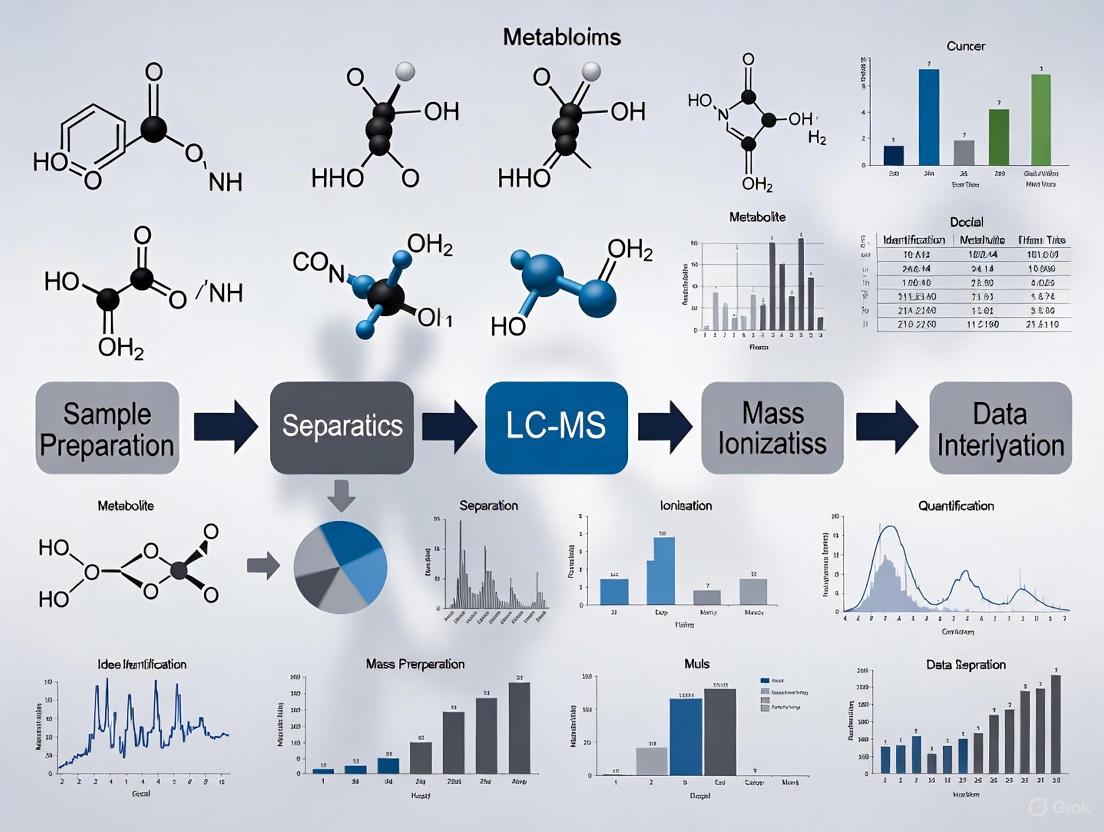
The entire LC-MS metabolomics process, from sample collection to data sharing, can be visualized as a cohesive workflow where each stage builds upon the previous one. The following diagram illustrates the logical sequence and interconnections between these critical phases:

Workflow Stages and Methodologies

Stage 1: Study Design

Objective: A well-structured study design is foundational for generating reliable, statistically robust, and interpretable metabolomics data [12].

Protocol:

• Define Research Objective: Clearly articulate the biological question, whether investigating disease mechanisms, drug responses, or metabolic pathway alterations.
• Select Sample Groups: Determine appropriate control and experimental groups with sufficient sample size to achieve statistical power. Common designs include case-control, longitudinal, and cohort studies.
• Choose Biological Matrix: Select appropriate sample types (e.g., plasma, urine, tissue, cell culture) based on the research objective.
• Plan Analytical Approach: Decide between untargeted metabolomics (comprehensive profiling of all measurable metabolites) and targeted metabolomics (quantification of a predefined set of metabolites) [13].
• Incorporate Quality Control (QC): Plan for QC samples, including pooled quality control samples (pooled from all samples), process blanks, and authentic reference standards to monitor instrument performance and data quality throughout the acquisition sequence [12].

Stage 2: Sample Preparation

Objective: To efficiently extract metabolites while preserving their integrity and quantitatively representing the in vivo metabolic state [11] [12].

Protocol:

• Collection & Quenching: Collect samples under standardized conditions to minimize pre-analytical variability. Immediately quench metabolic activity using rapid cooling with liquid nitrogen or chilled organic solvents (e.g., methanol at -80°C) to halt enzyme activity and stabilize the metabolome [11] [12].
• Metabolite Extraction: Employ liquid-liquid extraction with organic solvents to precipitate proteins and isolate metabolites. The choice of solvent dictates metabolite coverage:
  • Biphasic solvents (e.g., Methanol/Chloroform/Water): Simultaneously extract polar (into the methanol/water phase) and non-polar metabolites (into the chloroform phase) [11].
  • Polar solvents (e.g., Methanol, Acetonitrile): Preferable for extracting hydrophilic metabolites like amino acids and sugars [11].
  • Non-polar solvents (e.g., MTBE, Chloroform): Optimal for comprehensive lipidomics analysis [11].
• Add Internal Standards: Spike labeled isotope internal standards into the extraction solvent prior to sample processing. These standards correct for variability in extraction efficiency, matrix effects, and instrument performance, enabling accurate quantification [11].
• Purification & Derivatization: Remove particulate matter via filtration or centrifugation. Derivatization is less common in LC-MS than in GC-MS but may be used to enhance detection for specific compound classes.

Table 1: Common Metabolite Extraction Solvents and Applications

Solvent Type	Examples	Target Metabolites	Characteristics
Polar	Methanol, Acetonitrile, Water	Amino acids, sugars, nucleotides, organic acids	High polarity, miscible with water, effective for polar metabolites [11]
Non-polar	Chloroform, MTBE, Hexane	Lipids, fatty acids, sterols, hormones	Hydrophobic, effective for lipophilic compounds [11]
Biphasic/Mixed	Methanol/Chloroform/Water, Methanol/Isopropanol/Water	Broad-range, polar and non-polar	Combination of polar and non-polar properties for comprehensive extraction [11]

Stage 3: Data Acquisition

Objective: To separate, detect, and measure the mass-to-charge ratio (m/z) and intensity of metabolites in the sample extracts [12].

Protocol:

• Chromatographic Separation: Utilize Liquid Chromatography (e.g., Reversed-Phase, HILIC) to separate metabolites based on chemical properties like polarity, reducing ion suppression and complexity for the mass spectrometer.
• Mass Spectrometry Detection: Analyze metabolites using high-resolution mass spectrometers (e.g., Q-TOF, Orbitrap) for untargeted discovery, or triple-quadrupole instruments (e.g., QqQ) for targeted, high-sensitivity quantification in MRM mode [13].
• Quality Control During Acquisition: Intersperse QC samples throughout the analytical batch:
  • Pooled QC Samples: Analyze a sample pooled from all aliquots every 4-10 injections to monitor instrument stability, signal drift, and reproducibility.
  • Blanks: Run solvent blanks to identify background contamination and carryover.
  • Reference Standards: Use authentic chemical standards for quality control and retention time calibration.

Stage 4: Data Processing

Objective: To convert raw instrumental data into a structured data matrix of features (m/z and retention time pairs) with aligned intensities across all samples [12].

Protocol:

• Peak Picking & Deconvolution: Use software (e.g., XCMS, Progenesis QI, MassHunter) to detect chromatographic peaks and resolve co-eluting ions [14] [13].
• Retention Time Alignment & Peak Matching: Correct for minor shifts in retention time across samples and align features to ensure each metabolite is represented by the same data point in all samples.
• Normalization & Batch Correction: Apply statistical methods to correct for systematic variation from technical artifacts (e.g., instrument drift, batch effects) and biological confounding factors (e.g., urine dilution) [12].
• Imputation: Handle missing values using strategies such as replacement by a minimum value or k-nearest neighbors (KNN) imputation.

Stage 5: Metabolite Identification

Objective: To annotate and identify statistically significant features from the processed data matrix, linking them to known chemical structures [12].

Protocol:

• Spectral Matching: Compare experimental MS/MS spectra against reference spectral libraries (e.g., MassBank, HMDB, GNPS, METLIN). A high spectral match provides a confident annotation [12] [13].
• Database Search by Accurate Mass: Query compound databases using the accurately measured m/z value (typically with mass accuracy < 5-10 ppm) to generate a list of candidate metabolites [13].
• Confidence Levels: Report identification confidence based on the Metabolomics Standards Initiative (MSI) guidelines:
  • Level 1: Identified - Matched by two or more orthogonal properties (e.g., accurate mass and MS/MS spectrum) to an authentic standard analyzed in the same laboratory.
  • Level 2: Putatively Annotated - Based on spectral similarity to a public library.
  • Level 3: Putatively Characterized Compound Class - Based on physicochemical properties or spectral similarity to a characteristic compound class.
  • Level 4: Unknown - Distinct but unidentifiable metabolite [12].

Stage 6: Biomarker Identification and Statistical Analysis

Objective: To uncover metabolites that are statistically significantly altered between experimental conditions and have potential diagnostic, prognostic, or therapeutic value.

Protocol:

• Univariate Statistics: Apply t-tests (for two groups) or ANOVA (for multiple groups) to find metabolites with significant abundance changes. Correct for multiple testing using False Discovery Rate (FDR) control [14] [12].
• Multivariate Statistics:
  • Unsupervised (e.g., PCA): Used for exploratory data analysis to identify natural clustering, trends, and outliers without prior class labeling [13].
  • Supervised (e.g., PLS-DA, OPLS-DA): Used to maximize separation between pre-defined classes and identify features most responsible for the discrimination [14].
• Data Visualization: Utilize specific plots to interpret statistical results:
  • Volcano Plot: Visualizes the relationship between statistical significance (-log₁₀(p-value)) and the magnitude of change (logâ‚‚(Fold Change)), highlighting metabolites that are both statistically significant and biologically relevant [14] [13].
  • Heatmaps: Display the relative abundance of significant metabolites across all samples, often combined with hierarchical clustering to group metabolites with similar profiles [13].
• Machine Learning: Employ algorithms like Random Forest or Support Vector Machines (SVM) for robust biomarker discovery and classification model building [12].

Stage 7: Pathway Interpretation and Integration

Objective: To place the list of significant metabolites and identified biomarkers into a biological context by mapping them onto metabolic pathways.

Protocol:

• Pathway Analysis: Use enrichment analysis (e.g., with MetaboAnalyst) to identify biochemical pathways (from databases like KEGG, Reactome) that are significantly overrepresented in the dataset [12].
• Integration with Other Omics: Correlate metabolomics data with genomics, transcriptomics, and proteomics datasets to obtain a systems-level understanding of biological processes [12].

Stage 8: Data Sharing and Reproducibility

Objective: To ensure the transparency, reproducibility, and reusability of metabolomics data by the scientific community.

Protocol:

• Adhere to the FAIR Principles (Findable, Accessible, Interoperable, Reusable) [12].
• Submit raw and processed data, along with comprehensive metadata (experimental design, sample preparation, analytical methods), to public repositories such as MetaboLights or the Metabolomics Workbench [12].
• Follow community reporting standards for metabolite identification confidence [12].

The Scientist's Toolkit: Essential Research Reagents and Materials

Table 2: Key Reagents and Materials for LC-MS Metabolomics

Item	Function/Application	Examples & Notes
Internal Standards (Isotope-Labeled)	Correct for technical variability; enable absolute quantification.	¹³C, ¹⁵N-labeled amino acids, lipids; added prior to extraction [11].
Solvents for Extraction	Protein precipitation and metabolite extraction.	LC-MS grade Methanol, Acetonitrile, Chloroform, Water; form biphasic systems [11].
Authentic Chemical Standards	Metabolite identification (Level 1 confidence) and quantification.	Purchase pure compounds for definitive confirmation of retention time and fragmentation [12].
Quality Control Materials	Monitor instrument performance and data quality.	Pooled QC samples, process blanks, and commercial standard mixes [12].
Chromatography Columns	Separate metabolites prior to MS detection.	Reversed-Phase (C18), HILIC; choice depends on metabolite polarity of interest.
Amisulbrom	Amisulbrom, CAS:348635-87-0, MF:C13H13BrFN5O4S2, MW:466.3 g/mol	Chemical Reagent
Amitifadine	Amitifadine|Triple Reuptake Inhibitor|Research Use Only	Amitifadine is a serotonin–norepinephrine–dopamine reuptake inhibitor (SNDRI) for research. This product is for Research Use Only and not for human consumption.

This application note provides a detailed, step-by-step protocol for the complete LC-MS metabolomics workflow. By adhering to this structured framework—emphasizing rigorous study design, robust sample preparation, comprehensive data processing, and confident metabolite identification—researchers can generate high-quality, reproducible data. The integration of statistical analysis and pathway interpretation ultimately transforms raw spectral data into profound biological insights, accelerating discovery in drug development and biomedical research.

In liquid chromatography-mass spectrometry (LC-MS) metabolomics research, the reliability and validity of findings hinge on a foundation of robust experimental design. The inherent complexity of biological samples, technical variability in analytical platforms, and the multifactorial nature of metabolic responses demand rigorous methodological planning. This document outlines application notes and detailed protocols for three critical steps: determining sample size, implementing proper replication, and executing randomization procedures. Adherence to these principles is mandatory for generating statistically sound, reproducible, and biologically meaningful data in drug development and basic research.

Determining Sample Size for Sufficient Statistical Power

Key Concepts and Definitions

Selecting an appropriate sample size is a critical step that ensures your study has a high probability of detecting scientifically meaningful effects, a property known as statistical power [15]. An underpowered study (with too small a sample size) risks missing true biological effects (Type II errors), while an overly large sample wastes resources and may expose subjects to unnecessary risks [15]. The goal is to find a balance that allows for the detection of meaningful differences with high confidence.

The following parameters are essential for any sample size calculation [16] [15] [17]:

• Statistical Power (1-β): The probability that the test will correctly reject a false null hypothesis (i.e., find a difference when one truly exists). Typically set at 80% or 90%.
• Significance Level (α): The probability of rejecting a true null hypothesis (Type I error, or false positive). Usually set at 0.05 (5%).
• Effect Size: The minimum magnitude of difference or relationship that you want to be able to detect, and that is considered biologically or clinically relevant.
• Population Variability (Standard Deviation): An estimate of the expected variance in your data. This can be obtained from pilot data, previous literature, or estimated.

Application Protocol: Sample Size Calculation for LC-MS Metabolomics

This protocol provides a step-by-step guide for performing an a priori sample size calculation, suitable for a grant application or study plan.

• Step 1: Define the Primary Hypothesis and Analysis Method. Clearly state the primary comparison (e.g., control vs. treated group). The statistical test you plan to use (e.g., t-test, ANOVA, correlation) will determine the exact formula.
• Step 2: Estimate Variability. Use the standard deviation (SD) of your metabolomic feature of interest from a pilot study or prior similar work. If no data is available, use a conservative estimate. High variability requires a larger sample size.
• Step 3: Define the Meaningful Effect Size. Determine the minimum fold-change or difference in metabolite abundance that is biologically significant in your context. A smaller, more precise effect size requires a larger sample.
• Step 4: Set Power and Significance Levels. Conventionally, use a power of 80% or 90% and an alpha of 0.05.
• Step 5: Calculate Sample Size. Use statistical software (e.g., G*Power, R, PASS) or the formula below for a two-group comparison using a t-test:

n = [ (Z_{α/2} + Z_{β})^2 * (σ_1^2 + σ_2^2) ] / Δ^2

Where:

• n = sample size per group
• Z_{α/2} = Z-value for the desired alpha (1.96 for α=0.05)
• Z_{β} = Z-value for the desired power (0.84 for 80% power)
• σ_1, σ_2 = estimated standard deviations of the two groups
• Δ = the desired effect size to detect

• Step 6: Account for Attrition. Increase the calculated sample size by 10-20% to compensate for potential sample loss, analytical dropouts, or poor data quality.

Table 1: Example Sample Size Requirements for a Two-Group Comparison (t-test) Assumptions: Power=80%, α=0.05, Equal Group Sizes, SD=1.0

Effect Size (Δ)	Sample Size per Group	Total Sample Size
0.5	64	128
1.0	16	32
1.5	8	16
2.0	5	10

The Scientist's Toolkit: Reagents for Sample Size and Power Analysis

Tool / Reagent	Function in Experimental Design
G*Power Software	Free, dedicated software for calculating statistical power and required sample size for a wide range of tests [15].
Pilot Study Materials	Biological reagents and LC-MS consumables used to run a small-scale preliminary experiment to estimate population variability.
R / Python Statistical Packages	Programming environments with extensive libraries (e.g., pwr in R) for complex or custom sample size calculations.
Internal Metabolomic Database	A historical repository of experimental data from your lab, used to inform realistic estimates of effect sizes and variability.
Amitivir	Amitivir (CAS 111393-84-1) - Research Chemical
Bms-066	Bms-066, CAS:914946-88-6, MF:C19H21N7O2, MW:379.4 g/mol

Implementing Replication Strategies

Understanding Types of Replication

Replication is the repetition of experimental units or measurements to estimate variability and improve the reliability of inferences. In LC-MS metabolomics, it is critical to distinguish between different types of replication [18].

• Technical Replication: The same biological sample is prepared and/or analyzed multiple times. This helps quantify the variability introduced by the LC-MS platform, sample preparation, and data processing.
  • Example: Injecting the same pooled quality control (QC) sample multiple times throughout the run.
• Biological Replication: Different biological subjects (or cultures, etc.) are assigned to the same experimental condition. This accounts for the natural variation within a population and is essential for making inferences about the broader biological population.
  • Example: Using 10 different mice from the same strain and treatment group, rather than taking 10 technical measurements from one mouse.

True replication involves applying the same treatment to more than one independent experimental unit. Pseudo-replication, such as making multiple measurements from the same biological subject and treating them as independent, is a common flaw that inflates false confidence [18].

Application Protocol: Designing a Replication Scheme

This protocol ensures that your replication strategy adequately addresses both technical and biological variability.

• Step 1: Define the Experimental Unit. Identify the smallest independent entity to which a treatment is applied (e.g., a single mouse, a single cell culture flask). This dictates what constitutes a biological replicate.
• Step 2: Prioritize Biological Replication. The primary goal is to draw conclusions about a population. Therefore, the budget and resources should first be allocated to a sufficient number of biological replicates, as determined by the sample size calculation.
• Step 3: Incorporate Technical Replication Strategically.
  • Replication of Sample Preparation: Process each biological sample independently at least once. Duplicate preparations for a subset of samples can help quantify preparation variance.
  • Replication of LC-MS Analysis: The primary technical replication in metabolomics is the repeated analysis of pooled QC samples. These are used to monitor instrument stability, perform batch correction, and model technical variance. It is not necessary to inject every biological sample multiple times.
• Step 4: Randomize the Order. To prevent confounding, the order of sample preparation and MS injection for all biological and technical replicates must be randomized (see Section 4).

The workflow below illustrates the relationship between biological and technical replicates in a typical LC-MS metabolomics experiment:

Randomization Procedures to Control Bias

The Role of Randomization

Randomization is the cornerstone of a valid experiment. It involves allocating experimental units to treatment groups, or ordering analytical runs, using a random mechanism [18] [19]. Its primary purpose is to prevent bias and control for unknown or unmeasured confounding variables (e.g., instrument drift, subtle environmental changes, researcher bias) by spreading their potential effects evenly across all groups [18] [20]. Without randomization, treatment effects can become confounded with other factors, rendering conclusions unreliable [18].

Application Protocol: Randomization in Metabolomic Workflow

This protocol details how to implement randomization at key stages of an LC-MS metabolomics study.

• Step 1: Random Assignment of Subjects to Treatment Groups.

  • Method: Use a computer-generated random number sequence or a dedicated randomization module in statistical software. Do not allocate based on convenience or subjective judgment.
  • Consider Block Randomization: For small studies or to ensure perfect balance over time, use block randomization. This ensures that after every few subjects, the number assigned to each group is equal [19] [20]. Vary the block size to maintain unpredictability.

• Step 2: Randomize the Sample Preparation Order.

  • After biological samples are collected, the order in which they are processed (e.g., protein precipitation, centrifugation, dilution) should be fully randomized. This prevents batch effects in preparation from being systematically linked to a specific treatment group.

• Step 3: Randomize the LC-MS Analysis Order.

  • This is critical. The sequence in which samples are injected into the LC-MS must be random. A completely randomized design is ideal but can be logistically challenging [21].
  • Practical Alternative: Randomized Block Design: If the experiment must be run over several days (batches), treat "Day" or "Batch" as a blocking factor. Then, randomize the order of samples within each batch. This accounts for day-to-day instrumental variation [18] [21]. Pooled QC samples should be interspersed throughout each batch.

Table 2: Comparison of Randomization Methods for LC-MS Run Order

Method	Description	Advantages	Disadvantages
Complete Randomization	Every sample is assigned a random position in the injection sequence with no restrictions.	Simple, eliminates bias and confounding.	May not balance group representation across an instrument drift gradient.
Randomized Block Design	Samples are grouped into batches (blocks), and randomization occurs within each batch.	Controls for known sources of variability like day or batch effects [18].	Requires careful planning; the blocking factor must be included in final statistical models.
Stratified Randomization	Used when assigning subjects to groups; ensures balance of a key covariate (e.g., sex, baseline weight).	Increases comparability of groups for known important factors [19].	Increases complexity, especially with multiple stratification factors.

The following diagram summarizes the key stages of the LC-MS metabolomics workflow where randomization and replication must be applied:

In liquid chromatography-mass spectrometry (LC-MS) metabolomics, the pre-analytical phase—encompassing sample collection, handling, and storage—is a fundamental determinant of data quality and reliability. Inappropriate sample collection or storage can introduce high variability, instrument interferences, or metabolite degradation, ultimately compromising data integrity and reproducibility [22]. The reproducibility crisis in biomedical research, notably affecting fields like oncology and psychology, underscores the necessity of rigorous standard operating procedures (SOPs) [23]. This protocol details evidence-based procedures for collecting and handling common biological matrices to minimize pre-analytical variation and ensure the generation of robust, reproducible LC-MS metabolomics data.

Key Pre-Analytical Considerations for Experimental Design

Biological and Environmental Factors

Two fundamental biological factors must be considered during study design, as they significantly influence the metabolome:

• Nutritional Status: The metabolic state of a subject (fed vs. fasting) drastically alters biofluid and tissue metabolomes. For instance, in rodents, 16-hour fasting affects one-third to one-half of monitored serum metabolites, increasing fatty and bile acids while decreasing diet- and gut microbiota-derived metabolites [22]. Fasting plasma is typically used to explore systemic metabolic differences between populations.
• Circadian Rhythms: A large fraction of mammalian metabolism undergoes circadian oscillations. In mice, over 40% of the serum metabolome and 45% of the hepatic metabolome are sensitive to time of day, providing complementary information [22]. Time of collection must be carefully chosen and kept consistent across study days.

General Principles for Sample Handling

The following general principles apply to the handling of all biological matrices in metabolomics studies [22]:

• Temperature Control: During collection, samples must be kept at the lowest possible temperature. Immediate snap-freezing is recommended to quench enzymatic activity and prevent oxidation of labile metabolites.
• Aliquoting: Samples should be aliquoted whenever possible to avoid repeated freeze-thaw cycles, which cause progressive loss of sample quality.
• Long-Term Storage: For long-term preservation before analysis, storage at -80 °C or lower is essential.

Matrix-Specific Collection and Handling Protocols

Blood-Derived Samples (Plasma/Serum)

Blood is a highly informative but metabolically active biofluid that requires rapid processing.

Detailed Protocol:

• Collection: Draw blood into appropriate vacutainers (e.g., EDTA or heparin tubes for plasma; clot activator tubes for serum).
• Processing:
  • For Plasma: Centrifuge whole blood at 1,500-2,000 x g for 10 minutes at 4°C within 30 minutes of collection. Carefully collect the supernatant (plasma) without disturbing the buffy coat.
  • For Serum: Allow blood to clot at room temperature for 30 minutes, then centrifuge at 1,500-2,000 x g for 10 minutes at 4°C. Collect the supernatant (serum).
• Storage: Immediately aliquot the plasma/serum into cryovials and snap-freeze in liquid nitrogen. Store at -80°C [22] [24].

Urine

Urine is non-invasively collected and provides a historical overview of metabolic events but contains residual enzymatic activity.

Detailed Protocol:

• Collection: Collect urine into sterile containers. Choose between timed collection (to capture specific metabolic events) or 24-hour collection (to eliminate diurnal variability) based on the research question [22].
• Processing: Centrifuge at 2,000-3,000 x g for 10 minutes at 4°C to remove cells, bacteria, and debris. Collect the supernatant.
• Storage: Aliquot the supernatant into cryovials and snap-freeze for storage at -80°C [22].

Tissues (e.g., Liver)

Tissues are highly susceptible to post-collection metabolic changes and require immediate quenching of metabolism.

Detailed Protocol:

• Collection: Rapidly dissect the tissue of interest.
• Quenching and Washing: Immediately rinse the tissue with ice-cold saline or buffer to remove blood. For immediate metabolism quenching, submerge the tissue in liquid nitrogen. Alternatively, use a metal block cooled by liquid nitrogen [22].
• Storage: Store the snap-frozen tissue specimen at -80°C. For homogenization, perform the process under controlled, cold conditions using a bead beater or homogenizer while keeping samples on ice.

Feces

Fecal metabolome serves as a functional readout of gut microbiome activity and is highly sensitive to nutritional challenges [22].

Detailed Protocol:

• Collection: Collect feces into pre-weighed, sterile tubes.
• Homogenization and Aliquotting: For a representative profile, homogenize the entire stool sample or multiple random portions from the specimen before aliquotting.
• Storage: Immediately snap-freeze aliquots and store at -80°C [22].

Cell Cultures

Cell cultures require rapid metabolism quenching to capture the intracellular metabolome accurately.

Detailed Protocol:

• Quenching: At the desired time point, rapidly remove the culture medium. Quench metabolism immediately by washing cells with ice-cold saline and adding a cold extraction solvent (e.g., 80% methanol). Alternatively, directly scrape cells into a cold extraction solvent.
• Collection: Transfer the cell extract containing the metabolites to a tube.
• Storage: Snap-freeze the extracts and store at -80°C [22].

The following workflow summarizes the critical steps from sample collection to data processing:

Figure 1: Workflow for Reproducible Metabolomics Sample Management. This diagram outlines the critical stages from study design to data processing, highlighting steps essential for minimizing degradation and ensuring reproducibility.

Ensuring Reproducibility Through QC and Data Processing

Implementing Quality Control (QC)

Robust quality control is non-negotiable for reproducible metabolomics.

• Internal Standards: Add known amounts of stable isotope-labeled or chemical analogs of endogenous metabolites to all samples during extraction. This corrects for variability in sample preparation and instrument analysis [24].
• Pooled QC Samples: Create a pooled QC sample by combining equal aliquots from all study samples. This pooled QC is analyzed repeatedly throughout the analytical sequence to monitor instrument stability and perform data normalization, correcting for signal drift [25] [24].

Reproducible Data Processing

The choice of data processing software and parameters significantly impacts results. Inconsistency in tools like XCMS and MZmine has been a major roadblock, with studies showing that over half of the features detected may not be shared between different software tools [26].

• Trackable Data Processing: Modern tools like asari are designed with explicit algorithmic frameworks for better provenance tracking. Asari employs a "mass track" concept, performing mass alignment before elution peak detection, which helps avoid errors in feature correspondence common in other software [26].
• Reproducibility Assessment: Statistical methods like the MaRR (Maximum Rank Reproducibility) procedure can be applied to assess the consistency of metabolite measurements across technical or biological replicate samples. This non-parametric approach helps distinguish reproducible from irreproducible signals without relying on strict distributional assumptions [25].

The Scientist's Toolkit: Essential Reagents and Materials

Table 1: Essential Materials for LC-MS Metabolomics Sample Preparation.

Item	Function	Key Considerations
Cryogenic Tubes	Long-term sample storage at -80°C.	Use sterile, DNase/RNase-free tubes that can withstand ultra-low temperatures without cracking.
Internal Standards	Correction for technical variability during quantification.	Use a mixture of stable isotope-labeled compounds not expected to be in the sample.
Cryoprotectants	Protect tissue integrity during freezing.	Options include sucrose, DMSO, or glycerol for specific sample types.
Protein Precipitation Solvents	Deproteinization of samples (e.g., plasma).	Cold methanol, acetonitrile, or methanol/acetonitrile mixtures are commonly used.
Solid-Phase Extraction (SPE) Cartridges	Clean-up and fractionation to reduce matrix effects.	Select sorbent chemistry (e.g., C18, HILIC) based on the metabolite class of interest.
Bms 180742	Bms 180742, CAS:138828-04-3, MF:C67H93N11O22, MW:1404.5 g/mol	Chemical Reagent
BMS-303141	BMS-303141, CAS:943962-47-8, MF:C19H15Cl2NO4S, MW:424.3 g/mol	Chemical Reagent

Troubleshooting Common Pre-Analytical Challenges

Table 2: Common Pre-Analytical Challenges and Solutions.

Challenge	Impact on Data	Recommended Solution
Metabolite Degradation	Loss of labile metabolites, introduction of degradation artifacts.	Maintain cold chain; rapid snap-freezing; use protease/inhibitor cocktails for specific pathways.
Matrix Effects	Ion suppression/enhancement during MS analysis, reducing accuracy.	Sample clean-up (e.g., SPE, filtration); use of appropriate internal standards.
Batch Variability	Introduces non-biological variance that can obscure true effects.	Randomize sample processing order; use pooled QC samples for batch normalization.
Poor Reproducibility	Inability to replicate findings within or across labs.	Adhere to detailed SOPs; implement comprehensive QC; use trackable data processing software.

Reproducibility in LC-MS metabolomics is not a single step but a philosophy integrated throughout the entire workflow, beginning the moment a sample is collected. By rigorously controlling for biological variables like nutritional status and circadian rhythm, adhering to matrix-specific SOPs for collection and storage, implementing a robust QC system, and utilizing transparent data processing tools, researchers can significantly minimize degradation and variability. These practices form the foundation upon which reliable and impactful metabolomics science is built, ultimately fostering greater trust and enabling more rapid advancement in biomedical research and drug development.

Liquid chromatography-mass spectrometry (LC-MS) has emerged as the cornerstone technique for global metabolomics, enabling the detection of hundreds to thousands of metabolites in a single analytical run [27]. The success of any LC-MS metabolomics study is fundamentally dependent on the sample preparation step, particularly the extraction protocol, which directly influences metabolite coverage, data quality, and analytical reproducibility [27]. Biological samples such as plasma and serum contain proteins and phospholipids that can interfere with LC-MS analysis by causing ion suppression, enhancing matrix effects, and accelerating chromatographic column deterioration [28].

This application note systematically compares three principal extraction methodologies—solvent precipitation, liquid-liquid extraction (LLE), and solid-phase extraction (SPE)—within the context of LC-MS metabolomics protocol research. We provide a detailed comparative analysis based on quantitative performance metrics and offer optimized experimental protocols to guide researchers in selecting and implementing the most appropriate extraction strategy for their specific research objectives. The selection of an optimal extraction method must balance multiple factors, including metabolite coverage, reproducibility, recovery efficiency, and matrix effect minimization [27] [28].

Comparative Analysis of Extraction Techniques

The table below summarizes the key performance characteristics of the three primary extraction methods based on comparative studies in human plasma and serum.

Table 1: Comparison of Metabolite Extraction Methods for LC-MS Metabolomics

Extraction Method	Metabolite Coverage	Recovery Efficiency	Matrix Effects	Method Repeatability	Sample Consumption	Processing Time
Solvent Precipitation	Broadest coverage [27]	Excellent accuracy [27]	High susceptibility [28]	Outstanding [27]	Moderate	Fastest
Liquid-Liquid Extraction	Complementary to solvent methods [28]	Good for lipophilic compounds [29]	Moderate to low [30]	Good	Low to moderate	Moderate
Solid-Phase Extraction	Selective coverage [27]	Variable by sorbent [28]	Lowest [28]	Low reproducibility risk [27]	Highest	Longest

Detailed Method Comparison

Solvent Precipitation remains the most widely used extraction technique in global metabolomics due to its broad metabolite coverage and simplicity [27]. Methanol and methanol/acetonitrile mixtures demonstrate outstanding accuracy and are considered benchmark methods for metabolomics studies [27]. However, this broad specificity results in highly complex samples that can hinder the detection of low abundance metabolites and create significant matrix effects due to co-extraction of interfering compounds [28].

Liquid-Liquid Extraction offers an alternative approach that can provide complementary metabolite coverage when combined with solvent-based methods [28]. Methyl-tert-butyl ether (MTBE) has gained popularity for its ability to extract both polar and non-polar metabolites, demonstrating particular strength in lipidomics applications [28]. The selectivity of LLE can be finely tuned by manipulating solvent polarity and pH, allowing for targeted extraction of specific metabolite classes [29].

Solid-Phase Extraction provides the highest degree of selectivity among the three methods, resulting in significantly reduced matrix effects [28]. SPE methods, particularly mixed-mode phases combining reversed-phase and ion-exchange mechanisms, excel at removing phospholipids—major contributors to ion suppression in LC-MS analysis [30]. While SPE tends to reduce overall metabolite coverage compared to solvent precipitation, it offers superior sample clean-up and can be optimized for specific metabolite classes [27].

Table 2: Optimal Applications for Each Extraction Method

Research Objective	Recommended Method	Rationale
Global Untargeted Metabolomics	Methanol precipitation	Broadest metabolite coverage with excellent repeatability [27]
Targeted Analysis of Specific Metabolite Classes	Mixed-mode SPE	Enhanced selectivity and reduced matrix effects [30]
Lipidomics	MTBE LLE	Optimal recovery of both polar and lipid metabolites [28]
High-Throughput Screening	96-well plate protein precipitation	Rapid processing and easy automation [30]
Matrix-Sensitive Analyses	Phospholipid removal SPE	Significant reduction of ion suppression [30]

Experimental Protocols

Methanol-Based Solvent Precipitation Protocol

Principle: This method utilizes cold organic solvents to precipitate proteins while maintaining metabolite integrity, providing the broadest metabolite coverage for untargeted metabolomics [27].

Reagents and Materials:

• LC-MS grade methanol (pre-chilled to -20°C)
• Pooled human plasma or serum samples
• Internal standard mixture (e.g., stable isotope-labeled compounds)
• Microcentrifuge tubes (1.5 mL)
• Centrifuge capable of 14,000 × g
• Nitrogen evaporator
• Vortex mixer

Critical Steps and Optimization:

• Sample Preparation: Thaw plasma/serum samples on ice and vortex thoroughly before aliquoting.
• Precipitation: Maintain solvents at -20°C before use to ensure efficient protein precipitation and minimize enzymatic activity.
• Centrifugation: Ensure temperature-controlled centrifugation at 4°C to maintain metabolite stability.
• Reconstitution: Use initial mobile phase composition for reconstitution to ensure compatibility with LC-MS analysis.

Method Notes: This protocol demonstrates outstanding repeatability and is considered the gold standard for global metabolomics [27]. For enhanced coverage of lipids, a modified protocol using methanol/MTBE (1:3) can be employed [28].

Mixed-Mode Solid-Phase Extraction Protocol

Principle: Mixed-mode SPE utilizes sorbents with multiple retention mechanisms (reversed-phase and ion-exchange) to selectively isolate metabolite classes while effectively removing phospholipids and other interferents [30].

Reagents and Materials:

• Mixed-mode SPE cartridges (e.g., Oasis MCX or MAX, 30 mg/1 mL)
• LC-MS grade methanol, water, and ammonium hydroxide
• Formic acid (LC-MS grade)
• Vacuum manifold for SPE processing
• Nitrogen evaporator

Critical Steps and Optimization:

• Conditioning: Ensure proper cartridge conditioning to activate the sorbent for optimal recovery.
• Sample Loading: Dilute plasma with water (1:2) to ensure proper retention of polar metabolites.
• Selective Elution: Employ stepwise elution with pH adjustment to fractionate metabolite classes (acidic, basic, neutral).
• Eluate Handling: Evaporate eluents immediately after collection to prevent metabolite degradation.

Method Notes: Mixed-mode SPE provides excellent removal of phospholipids, significantly reducing matrix effects in LC-MS analysis [30]. While overall metabolite coverage may be lower than solvent precipitation, the improved data quality and reduced ion suppression make it ideal for targeted analyses [28].

Methyl-Tert-Butyl Ether (MTBE) Liquid-Liquid Extraction Protocol

Principle: MTBE-based LLE leverages the differential solubility of metabolites in immiscible solvents to extract both polar and non-polar compounds, making it particularly suitable for lipidomics and broad-spectrum metabolite analysis [28].

Reagents and Materials:

• LC-MS grade MTBE, methanol, and water
• Internal standard mixture
• Glass centrifuge tubes (recommended for organic solvents)
• Centrifuge capable of 3,000 × g
• Vortex mixer
• Nitrogen evaporator

Procedure:

• Sample Preparation: Aliquot 50 μL of plasma/serum into a glass centrifuge tube.
• Methanol Addition: Add 150 μL of methanol, vortex for 30 seconds to precipitate proteins.
• MTBE Addition: Add 500 μL of MTBE, vortex vigorously for 1 minute.
• Phase Separation: Add 125 μL of water to induce phase separation, vortex for 30 seconds.
• Centrifugation: Centrifuge at 3,000 × g for 10 minutes at 4°C.
• Fraction Collection:
  • Collect the upper organic phase (MTBE layer) containing lipids and non-polar metabolites.
  • Collect the lower aqueous phase (methanol/water layer) containing polar metabolites.
• Concentration: Evaporate both fractions to dryness under a stream of nitrogen.
• Reconstitution: Reconstitute the organic fraction in 50 μL isopropanol/acetonitrile (1:1) and the aqueous fraction in 50 μL initial mobile phase for LC-MS analysis.

Method Notes: MTBE extraction provides a comprehensive approach for simultaneous analysis of polar and non-polar metabolomes [28]. The partitioning behavior can be optimized by adjusting the ratio of organic to aqueous solvents based on the LogP values of target analytes [29].

The Scientist's Toolkit: Essential Research Reagents and Materials

Table 3: Essential Reagents and Materials for Metabolite Extraction

Item	Function	Application Notes
LC-MS Grade Methanol	Protein precipitant and extraction solvent	Provides broad metabolite coverage; pre-chill to -20°C for optimal protein precipitation [27] [31]
LC-MS Grade Acetonitrile	Protein precipitant	Effective for phospholipid removal; often used in combination with methanol [27] [30]
Methyl-Tert-Butyl Ether (MTBE)	LLE solvent	Excellent for simultaneous extraction of polar and non-polar metabolites [28]
Mixed-Mode SPE Cartridges	Selective metabolite isolation	Combine reversed-phase and ion-exchange mechanisms for enhanced selectivity [30]
Stable Isotope-Labeled Internal Standards	Quality control and quantification correction	Essential for monitoring extraction efficiency and correcting for matrix effects [32]
Formic Acid and Ammonium Hydroxide	pH adjustment for SPE	Critical for controlling ionization state and retention of metabolites in mixed-mode SPE [28]
Phospholipid Removal Plates	Specific phospholipid removal	Zirconia-coated silica plates selectively remove phospholipids to reduce matrix effects [30]
Bms493	Bms493, CAS:215030-90-3, MF:C29H24O2, MW:404.5 g/mol	Chemical Reagent
BMS-605541	BMS-605541, CAS:639858-32-5, MF:C19H17F2N5OS, MW:401.4 g/mol	Chemical Reagent

Method Selection and Integration Strategy

Decision Framework for Method Selection

Choosing the appropriate extraction method requires careful consideration of research goals, sample type, and analytical resources. The following framework provides guidance for method selection:

For Untargeted Discovery Studies: Methanol precipitation should be the default choice due to its extensive metabolite coverage and proven reliability [27]. The minimal sample manipulation preserves a comprehensive metabolite profile, making it ideal for hypothesis-generating research.

For Targeted Quantification: SPE methods, particularly mixed-mode approaches, offer superior performance for quantitative analysis by significantly reducing matrix effects and improving method sensitivity [30]. The selective nature of SPE provides cleaner extracts, resulting in enhanced signal-to-noise ratios for target analytes.

For Specialized Applications: LLE with MTBE excels in lipidomics and when analyzing both polar and non-polar metabolites simultaneously [28]. The ability to partition metabolites based on polarity facilitates class-specific analysis and can be further optimized using salting-out approaches (SALLE) for hydrophilic compounds [29].

Orthogonal Method Integration

For studies requiring maximal metabolome coverage, integrating multiple orthogonal extraction methods can significantly increase metabolite detection. Research demonstrates that combining methanol precipitation with ion-exchange SPE or MTBE LLE can increase metabolite coverage by 34-80% compared to any single method [28]. This approach, while increasing MS analysis time and sample consumption, provides the most comprehensive view of the metabolome.

The selection of an appropriate metabolite extraction strategy is a critical determinant of success in LC-MS metabolomics. Solvent precipitation methods, particularly methanol-based protocols, provide the broadest metabolite coverage and outstanding repeatability, making them ideal for untargeted discovery studies. SPE techniques offer enhanced selectivity and significantly reduced matrix effects, beneficial for targeted quantification. LLE methods, especially MTBE-based protocols, provide complementary coverage and are particularly well-suited for lipidomics applications.

Researchers should align their extraction strategy with specific research objectives, considering the trade-offs between metabolite coverage, matrix effects, and processing complexity. For the most comprehensive metabolomic analysis, integrating orthogonal extraction methods can substantially increase metabolite coverage, providing a more complete picture of the biological system under investigation.

Executing the LC-MS Workflow: From Sample Preparation to Data Acquisition

Liquid chromatography-mass spectrometry (LC-MS) metabolomics has become a cornerstone of modern biological and clinical research, providing a direct readout of physiological and pathological states by comprehensively measuring small molecules. The sample preparation stage, particularly metabolite extraction from complex biofluids like plasma, is a critical pre-analytical step that profoundly influences data quality, reproducibility, and biological interpretation. The selection of an appropriate extraction method must balance multiple competing factors: comprehensiveness of metabolite coverage, extraction efficiency, method repeatability, and the minimization of matrix effects [27] [33].

This application note systematically evaluates and compares seven solvent-based and solid-phase extraction methods for LC-MS metabolomics analysis of human plasma. Framed within a broader thesis on protocol standardization, this work provides researchers and drug development professionals with detailed, evidence-based protocols and performance data to facilitate the rational design of metabolomics workflows, thereby enhancing the impact and reliability of their research [27].

Critical Comparison of Extraction Method Performance

A rigorous assessment of seven common extraction methods was conducted using standard analytes spiked into both buffer and human plasma. The evaluated methods included three conventional solvent precipitations (Methanol, Methanol/Ethanol, Methanol/MTBE), one liquid-liquid extraction (LLE with MTBE), and three solid-phase extraction (SPE) protocols (C18, Mixed-Mode Ion-Exchange (IEX), and Divinylbenzene-Pyrrolidone (PEP2)) [28]. Performance was measured against key metrics including absolute recovery, matrix effects, repeatability, and metabolite coverage in combination with reversed-phase (RP) and mixed-mode (IEX/RP) LC-MS analyses.

Table 1: Comprehensive Performance Metrics of Seven Extraction Methods for Plasma Metabolomics

Extraction Method	Average Recovery (%)	Matrix Effects (Signal Suppression, %)	Method Repeatability (%RSD)	Metabolite Coverage	Key Strengths	Key Limitations
Methanol Precipitation	80-120 [34]	High [28]	Outstanding [27]	Broad, high for polar metabolites [27] [28]	Broad specificity, outstanding accuracy, simple protocol [27]	High matrix effects, highly complex sample [28]
Methanol/Ethanol Precipitation	Similar to Methanol [28]	High [28]	Excellent [28]	Wide, comparable to Methanol [28]	Excellent precision, wide selectivity [28]	High ion suppression
Methanol/MTBE Precipitation	Similar to Methanol [28]	High [28]	Excellent [28]	Wide [28]	Good for polar & lipid metabolomes [28]	High solvent consumption
MTBE LLE	Variable (6-93%) [35]	~50% post-EME [35]	2-15% [35]	Orthogonal to Methanol [28]	Good for polar & lipid metabolomes, robotic compatibility [28]	Variable recovery
C18 SPE	Selective	Lower than solvents [28]	Good [27]	Selective for non-polar metabolites	Reduced matrix effects, clean extracts	Lower overall metabolite coverage [27]
Mixed-Mode IEX SPE	Selective	Lower [28]	Good [27]	Orthogonal, good for ionic metabolites [28]	High orthogonality to solvent methods [27]	Low reproducibility risk, more selective [27]
PEP2 SPE	Selective	Lower [28]	Good [27]	Moderate	Reduced phospholipids, good repeatability [27]	More selective, lower coverage [27]

The data in Table 1 reveals that no single extraction method is superior across all metrics. Methanol-based solvent precipitation provides the best combination of broad metabolite coverage and high repeatability, confirming its status as a default method for global metabolomics [27] [28]. However, this broad specificity comes at the cost of significant matrix effects due to the co-extraction of interfering compounds, particularly phospholipids, which can suppress ionization of lower-abundance metabolites [28].

SPE methods, while generally more selective and resulting in lower metabolite coverage, produce cleaner extracts with significantly reduced matrix effects. Among SPE variants, mixed-mode IEX demonstrated the highest orthogonality to methanol-based methods, making it a strong candidate for sequential extraction protocols aimed at maximizing total metabolome coverage [28]. The MTBE-based LLE also showed good orthogonality and is particularly valuable for workflows targeting both polar and lipid metabolites [28].

Table 2: Orthogonality and Synergistic Potential of Extraction Methods

Method Combination	Increase in Metabolite Coverage vs. Best Single Method	Recommended Application
Methanol + IEX SPE	High	Maximizing coverage for discovery-phase studies
Methanol + MTBE LLE	High [28]	Integrated polar and lipid metabolomics
Methanol + C18 SPE	Moderate	Studies focusing on non-polar metabolite classes
Single Methanol Method	Baseline (0%)	High-throughput targeted analyses or resource-limited studies

The combination of multiple, orthogonal extraction methods can increase metabolome coverage by 34-80% compared to the best single extraction protocol, albeit with a corresponding increase in MS analysis time and sample consumption [28]. This strategy is particularly powerful for untargeted discovery-phase studies where comprehensive metabolite detection is the primary objective.

Detailed Experimental Protocols

Recommended Standardized Workflow

The following diagram illustrates the generalized workflow for metabolite extraction from plasma, common to all methods detailed in the subsequent sections.

Protocol 1: Methanol Precipitation (Monophasic)

This method is recommended for most untargeted profiling studies due to its broad specificity and high reproducibility [27].

• Step 1: Thaw plasma samples on ice or at 4°C. Vortex thoroughly before aliquoting.
• Step 2: Pipette 50 µL of plasma into a pre-cooled microcentrifuge tube.
• Step 3: Add 150 µL of cold (-20°C) LC/MS-grade methanol containing appropriate internal standards (e.g., stable isotope-labeled amino acids). Vortex vigorously for 30-60 seconds.
• Step 4: Incubate the mixture for 20 minutes at -20°C to facilitate protein precipitation.
• Step 5: Centrifuge at >14,000 × g for 15 minutes at 4°C.
• Step 6: Carefully transfer the supernatant to a new LC-MS vial. The pellet, containing precipitated proteins, is discarded.
• Step 7 (Optional): Evaporate the supernatant under a gentle stream of nitrogen or using a vacuum concentrator. Reconstitute the dried extract in a volume of initial mobile phase suitable for your LC-MS system (e.g., 100 µL of water:acetonitrile, 95:5). Vortex thoroughly before analysis.

Protocol 2: Matyash/MTBE Extraction (Biphasic)

This method is ideal for simultaneous extraction of polar metabolites and lipids, providing a more comprehensive view of the metabolome [36].

• Step 1: Aliquot 40 µL of plasma into a glass tube.
• Step 2: Add 150 µL of LC/MS-grade methanol (with 1 mM BHT as antioxidant) and spike with internal standards. Vortex well.
• Step 3: Add 500 µL of methyl tert-butyl ether (MTBE). Vortex continuously for 1 hour at room temperature.
• Step 4: Add 125 µL of LC/MS-grade water to induce phase separation. Vortex briefly and incubate on ice for 10 minutes.
• Step 5: Centrifuge at 2,000 × g for 10 minutes at room temperature. This will result in a three-phase system: a lower aqueous phase (polar metabolites), an upper organic phase (lipids), and a protein pellet at the interface.
• Step 6: Carefully collect the upper organic phase (lipids) and the lower aqueous phase (polar metabolites) into separate vials.
• Step 7: Dry both fractions under nitrogen or vacuum. Reconstitute each in solvents compatible with your chosen LC-MS method (e.g., methanol for lipids, water:acetonitrile for polar metabolites).

Protocol 3: Mixed-Mode Ion-Exchange (IEX) Solid-Phase Extraction

Use this method as an orthogonal technique to methanol precipitation to increase coverage of ionic metabolites [28].

• Step 1: Pre-condition the IEX SPE sorbent (e.g., divinylbenzene conjugated with sulfonic acid and quaternary amine moieties) with 1 mL of methanol.
• Step 2: Equilibrate the sorbent with 1 mL of water.
• Step 3: Load 50 µL of plasma (pre-diluted 1:1 with water or a weak acid/base depending on target metabolite class) onto the SPE cartridge.
• Step 4: Wash with 1-2 mL of water or a mild buffer (e.g., 5 mM ammonium acetate) to remove unretained neutral compounds and salts.
• Step 5: Elute retained metabolites sequentially using solvents of increasing strength and pH manipulation. A typical sequence might be:
  • Elution 1 (Acidic Analytics): 1 mL of methanol with 2% formic acid.
  • Elution 2 (Basic Analytics): 1 mL of methanol with 5% ammonium hydroxide.
• Step 6: Combine or keep separate eluates based on analytical needs. Dry under nitrogen or vacuum and reconstitute in LC-MS compatible solvent.

The Scientist's Toolkit: Essential Research Reagents & Materials

Successful and reproducible metabolomics sample preparation relies on the use of high-quality, MS-compatible materials. The following table lists essential reagents and materials.

Table 3: Essential Research Reagents and Materials for Plasma Metabolite Extraction

Item Name	Specification / Example	Critical Function	Notes for Use
Plasma Samples	Collected with EDTA or heparin anticoagulant; stored at -80°C	Primary biological matrix	Avoid repeated freeze-thaw cycles; thaw on ice [33]
LC-MS Grade Methanol	Optima LC/MS grade or equivalent	Primary extraction solvent, protein precipitation	High purity minimizes background interference
LC-MS Grade Acetonitrile	Optima LC/MS grade or equivalent	Modifies extraction selectivity	Often used in combination with methanol (e.g., 1:1) [27]
MTBE (Methyl tert-butyl ether)	HPLC grade or higher	Organic solvent for biphasic LLE	Less dense than water; organic layer forms on top [36]
Internal Standards	Stable isotope-labeled metabolites (e.g., L-Phenylalanine-d8, L-Valine-d8) [6]	Monitors extraction efficiency & data normalization	Should be added at the very beginning of extraction [6]
Formic Acid	Optima LC/MS grade, 99%+	Mobile phase additive, aids ionization	Typically used at 0.1% in mobile phases [6]
Ammonium Formate/Acetate	LC-MS grade, 99%+	Mobile phase buffer for improved chromatography	Typically used at 5-10 mM concentration [6]
SPE Cartridges	Mixed-mode IEX, C18, PEP2 chemistries	Selective clean-up and fractionation	IEX provides high orthogonality to solvent methods [28]
Amitriptyline	Amitriptyline|CAS 50-48-6|Research Chemical		Bench Chemicals
Ampicillin Trihydrate	Ampicillin Trihydrate	High-purity Ampicillin Trihydrate for research applications. For Research Use Only (RUO). Not for human, veterinary, or household use.	Bench Chemicals

The optimal choice of metabolite extraction method is dictated by the specific goals of the study. Based on the systematic comparison presented herein, the following evidence-based recommendations are proposed:

• For Global Untargeted Metabolomics: Methanol precipitation remains the recommended starting point due to its broad metabolite coverage, simplicity, and high reproducibility [27]. Researchers should be aware of its susceptibility to matrix effects and employ appropriate internal standards to correct for ionization suppression [28].
• For Maximum Metabolome Coverage: For discovery-phase research where comprehensiveness is the priority, a sequential extraction protocol combining methanol precipitation with an orthogonal method like mixed-mode IEX SPE or MTBE LLE is highly recommended. This approach can increase coverage by over 30% compared to a single method [28].
• For High-Throughput Targeted Analysis: Methanol precipitation is also suitable for targeted assays, but SPE methods or novel techniques like Electromembrane Extraction (EME) should be considered if the target analytes are known to suffer from significant matrix effects in solvent-only extracts [35]. EME, for instance, can drastically reduce matrix effects even with limited sample dilution [35].
• For Integrated Polar and Lipid Metabolomics: The Matyash/MTBE biphasic extraction provides a robust and efficient single-protocol solution for simultaneous preparation of both polar and lipid fractions, simplifying the workflow and reducing sample consumption [36].

In conclusion, the rational selection and application of these optimized extraction protocols, tailored to the analytical objectives, will significantly enhance the quality and biological relevance of data generated in LC-MS metabolomics studies, thereby strengthening the foundation for subsequent biomarker discovery, drug development, and clinical translation.

In liquid chromatography-mass spectrometry (LC-MS) metabolomics, the selection of the chromatographic mode is a fundamental determinant of the coverage and quality of the analytical data. Reversed-phase (RP) chromatography has long been the default mode for many LC-MS applications due to its robustness, high separation efficiency, and straightforward compatibility with electrospray ionization (ESI) [37]. However, its limitations in retaining highly polar metabolites have encouraged the adoption of alternative techniques. Hydrophilic interaction liquid chromatography (HILIC) has emerged as a powerful complementary technique, offering orthogonal selectivity for polar and ionizable compounds that are often poorly retained in RP [37]. A comprehensive LC-MS metabolomics protocol should leverage the strengths of both RP and HILIC to achieve maximal coverage of the metabolome, which encompasses a vast diversity of physicochemical properties [37] [38]. This application note provides a detailed comparison and protocols for implementing these two chromatographic modes.

Fundamental Principles and Separation Mechanisms

Reversed-Phase (RP) Chromatography

The retention mechanism in RP chromatography is primarily driven by hydrophobic interactions between analytes and the non-polar stationary phase. Common stationary phases include C18, C8, and phenyl columns. Analytes are eluted using a gradient that starts with a predominantly aqueous mobile phase and increases the proportion of an organic solvent, typically methanol or acetonitrile. This environment is highly compatible with ESI-MS, providing good ionization efficiency for a wide range of mid- to non-polar compounds [37].

Hydrophilic Interaction (HILIC) Chromatography

HILIC functions through a more complex, multimodal retention mechanism. It employs a polar stationary phase (e.g., bare silica, amide, zwitterionic) and a mobile phase with a high proportion of an organic solvent, usually acetonitrile. The primary mechanism is the partition of analytes between the bulk organic-rich mobile phase and a water-enriched layer that forms on the surface of the stationary phase [37] [39]. Additional interactions, such as ionic exchange, dipole-dipole interactions, and hydrogen bonding, also contribute to retention, depending on the stationary phase chemistry and mobile phase conditions [37] [40]. The high organic content of HILIC mobile phases enhances ESI-MS sensitivity by improving desolvation and ionization efficiency [37] [39].

Table 1: Core Principles of Reversed-Phase and HILIC Chromatography

Feature	Reversed-Phase (RP)	Hydrophilic Interaction (HILIC)
Retention Mechanism	Hydrophobic partitioning	Hydrophilic partitioning, hydrogen bonding, ionic interactions
Stationary Phase	Non-polar (C18, C8)	Polar (silica, amide, zwitterionic, diol)
Typical Mobile Phase	Water-methanol or water-acetonitrile gradient	High acetonitrile (60-95%) to aqueous buffer gradient [39]
Elution Order	Polar compounds elute first	Non-polar compounds elute first
Ideal for Analytes	Mid- to non-polar molecules	Polar and ionizable molecules [37]

Comparative Performance in Metabolomics Applications

Analyte Coverage and Selectivity

The orthogonality of RP and HILIC selectivity is their greatest advantage when used together. RP chromatography excels at separating lipids, non-polar secondary metabolites, and other hydrophobic compounds. In contrast, HILIC is indispensable for retaining polar metabolites such as amino acids, nucleosides, nucleotides, organic acids, saccharides, and neurotransmitters, which often elute in or near the void volume in RP [37] [40]. Research has shown that integrating HILIC-MS into a metabolomics workflow significantly broadens metabolome coverage compared to using reversed-phase LC-MS alone [37] [38].

Chromatographic Performance and Sensitivity

RP chromatography is generally characterized by high separation efficiency and sharp peak shapes, leading to high peak capacity [37] [41]. HILIC can sometimes suffer from broader peaks and longer equilibration times [37] [41]. However, regarding sensitivity, HILIC often provides an advantage for polar analytes. The organic-rich mobile phase promotes superior desolvation and ionization in the ESI source, frequently resulting in lower limits of detection for polar metabolites compared to RP [39]. A systematic evaluation found that HILIC conditions can lead to a substantial improvement in sensitivity for a large variety of compounds [39].

Matrix Effects and Practical Considerations

Matrix effects, the suppression or enhancement of ionization by co-eluting compounds, are a critical consideration in LC-MS. The extent of matrix effects is highly dependent on the sample matrix, sample clean-up, and chromatographic mode. One study systematically evaluated matrix effects in plasma and urine and found that the optimal combination of stationary phase and mobile phase pH differed between RPLC and HILIC [39]. HILIC can be particularly beneficial when coupled with simple protein precipitation, as the eluate is compatible with the high organic starting mobile phase, eliminating the need for solvent evaporation and reconstitution [39].

Table 2: Performance Comparison for Metabolomics

Performance Metric	Reversed-Phase (RP)	Hydrophilic Interaction (HILIC)
Peak Shape & Efficiency	Typically sharp peaks, high efficiency [41]	Can exhibit broader peaks; improved with additives like phosphate [37]
Sensitivity (ESI-MS)	Good for a wide range of compounds	Often enhanced for polar compounds due to high organic content [37] [39]
Equilibration Time	Relatively fast	Can be longer [41]
Tolerance to Sample Solvent	Critical (should be weak solvent)	Critical (should be strong solvent)
Handling of Matrix Effects	Well-documented; depends on cleanup	Can be different from RP; requires evaluation [39]

Experimental Protocols for LC-MS Metabolomics

Sample Preparation for Cultured Cells

The following protocol, adapted for targeted amino acid analysis, outlines a robust workflow for adherent mammalian cells [38].

• Quenching and Metabolite Extraction:

  • Aspirate the culture medium and quickly wash the cell layer with ice-cold saline solution.
  • Immediately add ice-cold 100% methanol (e.g., 1 mL per 10 cm² culture dish) to quench cellular metabolism.
  • While the dish is on a bed of ice, use a cell scraper to harvest the cells directly into the quenching solvent.
  • Transfer the cell suspension to a pre-cooled microcentrifuge tube.
  • Vortex thoroughly and incubate on dry ice or at -80°C for 10 minutes to complete protein precipitation.
  • Centrifuge at 4°C (e.g., 13,000-16,000 × g for 10-15 minutes) to pellet insoluble material and proteins.
  • Carefully collect the supernatant, which contains the extracted metabolites, into a new tube.

• Sample Normalization and Analysis:

  • Normalize the samples based on a parameter reflecting the original cell biomass, such as total protein content determined from a parallel cell culture.
  • Evaporate the solvent under a gentle stream of nitrogen or using a vacuum concentrator.
  • Reconstitute the dried metabolite extract in a solvent compatible with the subsequent LC-MS analysis. For HILIC, reconstitute in a high-ACN solvent (e.g., 80-90% ACN); for RP, reconstitute in a high-water solvent.

HILIC-MS Method for Targeted Amino Acid Analysis

This protocol provides a starting point for the separation and detection of underivatized amino acids, such as proline, arginine, and glutamic acid [38].

• Chromatography Conditions:

  • Column: Amide or zwitterionic HILIC column (e.g., 2.1 x 100 mm, 1.7-1.8 µm).
  • Mobile Phase A: Aqueous ammonium formate or ammonium acetate buffer (e.g., 5-50 mM, pH ~3-6).
  • Mobile Phase B: Acetonitrile.
  • Gradient: Begin with a high percentage of B (e.g., 85-95%), followed by a linear increase to a higher percentage of A over 10-20 minutes.
  • Flow Rate: 0.2-0.4 mL/min.
  • Column Temperature: 25-40°C.
  • Injection Volume: 1-5 µL.

• Mass Spectrometry Conditions:

  • Ionization: Electrospray Ionization (ESI), positive mode for amino acids.
  • Mass Analyzer: High-resolution, accurate-mass (HRAM) spectrometer (e.g., Orbitrap, Q-TOF).
  • Data Acquisition: Full-scan MS or targeted SIM/MS² for quantification and confirmation.

Reversed-Phase LC-MS Method for Broad Metabolite Profiling

This protocol describes a generic RP method suitable for a wide range of metabolites.

• Chromatography Conditions:

  • Column: C18 column (e.g., 2.1 x 100 mm, 1.7-1.9 µm).
  • Mobile Phase A: Water with 0.1% formic acid.
  • Mobile Phase B: Methanol or acetonitrile with 0.1% formic acid.
  • Gradient: Begin with a low percentage of B (e.g., 2-5%), ramp to a high percentage (e.g., 95-99%) over 10-20 minutes, hold, and re-equilibrate.
  • Flow Rate: 0.3-0.5 mL/min.
  • Column Temperature: 40-60°C.
  • Injection Volume: 1-5 µL.

• Mass Spectrometry Conditions:

  • Ionization: ESI, alternating between positive and negative modes.
  • Mass Analyzer: HRAM spectrometer.
  • Data Acquisition: Full-scan MS at high resolution for untargeted profiling.

Workflow Visualization and Decision Pathway

The Scientist's Toolkit: Essential Research Reagents and Materials

Table 3: Key Reagents and Materials for LC-MS Metabolomics

Item	Function/Description	Example Use Case
Ice-cold Methanol	Quenches metabolic activity and extracts metabolites.	Cell culture quenching and metabolite extraction [38].
Ammonium Formate/Acetate	MS-compatible volatile salts for mobile phase buffering.	Controlling pH and ionic strength in HILIC and RP mobile phases [38].
Formic Acid	Common mobile phase additive to promote protonation in ESI+.	Improving ionization and peak shape in RP chromatography.
HILIC Column (e.g., Amide)	Polar stationary phase for retaining hydrophilic analytes.	Separation of underivatized amino acids and polar metabolites [38].
RP Column (e.g., C18)	Hydrophobic stationary phase for retaining lipophilic analytes.	Separation of lipids and non-polar metabolites.
Phosphate Additive (µM)	Trace additive to shield electrostatic interactions in HILIC.	Improving peak shape for polar compounds on zwitterionic phases [37].
Amsilarotene	Amsilarotene, CAS:125973-56-0, MF:C20H27NO3Si2, MW:385.6 g/mol	Chemical Reagent
AMTB hydrochloride	AMTB hydrochloride, MF:C23H27ClN2O2S, MW:431.0 g/mol	Chemical Reagent

Reversed-phase and HILIC chromatographies are not competing techniques but rather complementary pillars of a comprehensive LC-MS metabolomics strategy. RP-LC remains the gold standard for non-polar to moderately polar metabolites, offering high efficiency and robustness. HILIC-LC is essential for capturing the highly polar fraction of the metabolome that is inaccessible to RP, while also offering potential gains in MS sensitivity. The orthogonal selectivity of these two modes makes their combined application the most effective approach for achieving extensive metabolome coverage, reducing analytical bias, and generating high-quality data for systems biology and biomarker discovery.

Liquid Chromatography-Mass Spectrometry (LC-MS) has become the primary analytical platform for global metabolomics due to its high throughput, soft ionization capabilities, and extensive coverage of metabolites [42] [43]. Metabolomics involves the comprehensive identification and quantification of small molecules (<1 kDa) in biological systems, providing a direct readout of biochemical activity and physiological status [44]. The success of LC-MS-based metabolomic studies depends on the appropriate selection and configuration of ionization sources and mass analyzers, which collectively determine the sensitivity, coverage, and quality of the metabolic data acquired [42]. This application note provides detailed technical protocols for configuring these critical components within the context of LC-MS metabolomics, supporting applications from basic research to drug discovery and development [44].

Electrospray Ionization (ESI)

Principle and Mechanism: Electrospray Ionization (ESI) uses electrical energy to assist the transfer of ions from solution into the gaseous phase [45]. The process involves three distinct stages: (1) dispersal of a fine spray of charged droplets through a capillary maintained at high voltage (typically 2.5-6.0 kV); (2) solvent evaporation aided by a heated drying gas (e.g., nitrogen), which increases the surface charge density as droplets shrink; and (3) ion ejection when the electric field strength within the charged droplet reaches a critical point, releasing ions into the gaseous phase [45] [46]. These ions are then sampled through a skimmer cone into the mass analyzer [45].

Key Characteristics: ESI is exceptionally suited for analyzing thermally labile and non-volatile biomolecules, including proteins, peptides, nucleotides, and most metabolites [45] [46]. A defining feature is its ability to generate multiple-charge ions, effectively extending the mass range of analyzers to accommodate kDa-MDa molecules [46]. As a soft ionization technique, it typically produces intact molecular ions with minimal fragmentation [42].

Table 1: Comparison of Common Ionization Sources in LC-MS Metabolomics

Parameter	ESI	APCI	APPI
Ionization Mechanism	Charge transfer in solution, followed by desolvation and ion evaporation [45] [46]	Gas-phase chemical ionization at atmospheric pressure via corona discharge [47] [48]	Gas-phase ionization through photon absorption and charge transfer [42]
Optimal Flow Rate	0.2-1.0 mL/min (nebulizer gas enhances higher flow rates) [45]	0.2-2.0 mL/min (compatible with standard-bore HPLC) [47]	Similar to APCI [42]
Polarity Compatibility	Excellent for polar and ionic compounds [42]	Suitable for medium to low polarity, thermally stable compounds [47] [42]	Best for non-polar compounds [42]
Molecular Weight Range	Up to 1,500 Da and beyond (including multiply charged biomolecules) [45] [46]	< 1,500 Da (typically produces singly charged ions) [47]	< 1,500 Da [42]
Fragmentation	Minimal (soft ionization) [46]	Minimal, but thermal degradation possible in heated nebulizer [47]	Minimal [42]
Key Applications in Metabolomics	Polar metabolites, organic acids, phospholipids, amino acids, peptides [45] [42]	Lipids, steroids, fatty acids, less polar secondary metabolites [47] [42]	Polyaromatic hydrocarbons, lipids, fat-soluble vitamins [42]

Atmospheric Pressure Chemical Ionization (APCI)

Principle and Mechanism: Atmospheric Pressure Chemical Ionization (APCI) utilizes gas-phase ion-molecule reactions at atmospheric pressure [47]. The LC effluent flows into a pneumatic nebulizer which creates a mist of fine droplets that are vaporized upon impact with heated walls (350-500°C) [47] [48]. The resulting vapor mixture is then directed past a corona discharge needle (maintaining a constant current of 2-5 µA), where the solvent molecules are ionized first [47]. These primary solvent ions subsequently react with analyte molecules through proton transfer or adduction processes to produce sample ions [47] [48]. In positive ion mode with water as the primary solvent, the ionization proceeds through a series of reactions beginning with N₂ ionization, leading to water cluster ions [H+(H₂O)ₙ] that ultimately protonate the analyte molecules (M) to form [M+H]⁺ ions [47].

Key Characteristics: APCI is particularly effective for analyzing less polar and thermally stable compounds with molecular weights below 1500 Da [47]. As it occurs in the gas phase after vaporization, APCI is more tolerant of non-polar solvents and higher buffer concentrations compared to ESI, making it more versatile for various reversed-phase LC conditions [47] [42]. The technique typically produces singly charged ions, resulting in simpler mass spectra compared to ESI [48].

Atmospheric Pressure Photoionization (APPI)

Principle and Mechanism: While detailed mechanisms of APPI are beyond the scope of this note, it shares the atmospheric pressure operation with APCI but uses a photon source (typically a krypton discharge lamp) instead of a corona discharge to initiate ionization [42]. The photons ionize dopant molecules or analytes directly, leading to charge transfer reactions that ultimately ionize the target molecules.

Key Characteristics: APPI is particularly complementary to ESI and APCI for analyzing non-polar compounds such as polyaromatic hydrocarbons and certain lipids that ionize poorly by the other techniques [42]. Its application range in terms of molecular weight and polarity is illustrated in Figure 1 alongside ESI and APCI.

Figure 1: Workflow Comparison of ESI, APCI, and APPI Ionization Processes

Mass Analyzers: Technical Specifications and Performance

Triple Quadrupole (QqQ)

Principle and Mechanism: The triple quadrupole mass analyzer consists of three sets of quadrupole rods arranged in series [45]. The first quadrupole (Q1) mass-selects precursor ions of interest, the second quadrupole (Q2) serves as a collision cell where collision-induced dissociation (CID) occurs with an inert gas such as argon, and the third quadrupole (Q3) analyzes the resulting product ions [45]. This configuration enables several specialized scanning modes essential for targeted metabolomics: Product Ion Scan (identifying fragments of a specific precursor), Precursor Ion Scan (finding all precursors that produce a specific fragment), Neutral Loss Scan (detecting all precursors that lose a common neutral fragment), and Multiple Reaction Monitoring (MRM) [45]. MRM is particularly valuable for quantitative analysis, offering exceptional specificity and sensitivity by monitoring specific precursor-product ion transitions [45].

Key Characteristics: Triple quadrupoles are robust, economical, physically compact, and readily interfaced with various inlet systems [45]. They excel in targeted quantitative analyses where high sensitivity and specificity are required, such as in pharmacokinetic studies and biomarker validation [45] [49]. While traditionally considered low-resolution instruments, recent advancements with post-acquisition calibration algorithms have demonstrated that accurate mass measurements (<10 mDa) are achievable, expanding their utility for molecular formula determination [49].

Quadrupole-Time of Flight (QTOF)

Principle and Mechanism: The QTOF mass analyzer combines a quadrupole mass filter with a time-of-flight (TOF) mass analyzer [49] [42]. The quadrupole component can operate in either RF-only mode to transmit all ions or as a mass filter to select specific precursor ions [42]. The TOF analyzer separates ions based on their velocity in a field-free drift region, with smaller ions reaching the detector first [42]. Modern QTOF instruments incorporate an orthogonal accelerator that pulses ions into the flight tube, along with an ion mirror (reflectron) that corrects for energy spread and improves resolution [42].

Key Characteristics: QTOF instruments provide high resolution (typically >17,000 FWHM for m/z 222) and accurate mass measurement capabilities (<5 ppm mass error) [49]. This enables precise elemental composition determination and facilitates the identification of unknown metabolites [42]. The hybrid design allows for MS/MS experiments with high mass accuracy in both MS and MS/MS modes, making QTOF particularly valuable for untargeted metabolomics and metabolite identification [49] [42].

Orbitrap

Principle and Mechanism: The Orbitrap mass analyzer is based on the Kingdon trap design, consisting of a central spindle-like electrode and two outer cup-like electrodes [50]. Ions are injected tangentially into the electric field between these electrodes and undergo stable rotational motion around the central electrode while simultaneously oscillating along the axial direction [50]. The frequency of these axial oscillations is mass-dependent and is detected by image current on the outer electrodes [50]. Fourier transformation of this signal yields the mass spectrum [50]. Orbitrap instruments are typically paired with a C-trap for ion accumulation and cooling before injection into the Orbitrap analyzer [50].

Key Characteristics: Orbitrap analyzers offer very high resolution (up to 500,000 FWHM), sub-ppm mass accuracy, and a dynamic range sufficient for metabolomic applications [42] [50]. The high mass stability and accuracy make them exceptionally well-suited for untargeted metabolomics where confident compound identification is crucial [42]. When coupled with ESI ionization, Orbitrap systems provide comprehensive coverage of the metabolome, enabling both discovery and targeted verification analyses within a single platform [50].

Table 2: Performance Comparison of Mass Analyzers in Metabolomics

Parameter	Triple Quadrupole (QqQ)	QTOF	Orbitrap
Resolution (FWHM)	Unit mass (≈500) [49]	High (≈17,000 for m/z 222) [49]	Very High (up to 500,000) [42]
Mass Accuracy	5-100 ppm (with calibration); <10 mDa achievable with post-processing [49]	<5 ppm [49]	<1 ppm [42]
Scan Speed	Fast for MRM transitions, slower for full scan	Fast (up to 100 Hz) [42]	Moderate (depends on resolution setting) [42]
Dynamic Range	5-6 orders of magnitude [45]	4-5 orders of magnitude [42]	4-5 orders of magnitude [42]
Fragmentation Capability	CID in RF-only collision cell [45]	CID, HCD available [42]	CID, HCD, ETD available [42]
Quantitation Performance	Excellent (MRM offers highest sensitivity and specificity) [45]	Good (wide dynamic range, high accuracy) [49]	Good (high resolution, accurate mass) [42]
Primary Metabolomics Applications	Targeted analysis, absolute quantitation, clinical biochemistry [45]	Untargeted profiling, metabolite identification, suspect screening [49] [42]	Untargeted profiling, unknown identification, pathway analysis [42]

Integrated LC-MS Workflows for Metabolomics

Experimental Design Considerations

A typical LC-MS metabolomics workflow encompasses experimental design, sample collection, metabolite extraction, LC-MS analysis, data processing, and functional interpretation [42] [43]. Proper experimental design is crucial, requiring sufficient biological replicates (minimum of three, with five preferred) to achieve adequate statistical power [42]. Incorporating quality control (QC) samples throughout the analytical sequence is essential for monitoring instrument performance and evaluating data quality [42]. Sample collection and handling must be standardized to minimize variability, with immediate storage at -80°C or in liquid nitrogen to prevent metabolite degradation [42].

Metabolite Extraction Strategies

Metabolite extraction represents a critical step that significantly influences experimental reproducibility and metabolome coverage [42]. The chemical diversity of metabolites necessitates optimized extraction protocols tailored to specific sample types and study objectives [42]. Common unbiased extraction methods include:

• Liquid-Liquid Extraction (LLE): Choice of solvents depends on metabolite chemical properties, with particular solvents extracting metabolites of similar chemical classes [42].
• Solid-Liquid Extraction (SLE): Requires optimization to avoid metabolite degradation, often needing multiple extraction steps or additional sample grinding for maximum recovery [42].
• Solid Phase Extraction (SPE): Effective for both sample extraction and removal of interfering substances, with various sorbents available including C-18, ion-exchange materials, and restricted access materials [42].

The selection of extraction method should be guided by performance evaluation of metabolite recovery, extraction specificity, and efficiency [42].

Figure 2: Integrated LC-MS Metabolomics Workflow from Sample to Interpretation

Data Acquisition and Processing

LC-MS data acquisition for metabolomics typically involves full-scan MS¹ analysis coupled with data-dependent (DDA) or data-independent (DIA) MS² acquisition [43]. Analysis in both positive and negative ionization modes across a mass range of m/z 50-1000 maximizes metabolome coverage [42]. Modern computational workflows such as MetaboAnalystR 4.0 provide integrated solutions for raw spectra processing, feature detection, compound identification, and statistical analysis [43]. For MS² data, efficient deconvolution algorithms are essential to address chimeric spectra in DDA and complex fragment-ion reassembly in DIA methods like SWATH-MS [43]. Compound identification relies on matching accurate mass, retention time, and fragmentation patterns against comprehensive reference databases containing >1.5 million spectra [43].

Experimental Protocols

Protocol 1: Untargeted Metabolomics Using ESI-QTOF

Objective: Comprehensive profiling of metabolites in biological samples for hypothesis generation.

Materials and Reagents:

• Extraction solvent: Methanol:Water (4:1, v/v) with internal standards
• Mobile phase A: 0.1% Formic acid in water
• Mobile phase B: 0.1% Formic acid in acetonitrile
• Quality control: Pooled quality control (QC) sample from all study samples

Instrumentation:

• LC System: UHPLC with C18 column (100 × 2.1 mm, 1.7 μm)
• Mass Spectrometer: QTOF instrument with ESI source
• Data Processing Software: MetaboAnalystR 4.0 [43] or equivalent

Procedure:

• Sample Preparation: Homogenize tissue or biofluid samples in extraction solvent (20:1 solvent-to-sample ratio) using bead-beating or vortexing. Centrifuge at 14,000 × g for 15 minutes at 4°C. Transfer supernatant to LC vials [42].
• LC Conditions: Maintain column temperature at 40°C. Use gradient elution: 5-95% B over 20 minutes. Flow rate: 0.4 mL/min. Injection volume: 5 μL [42].
• MS Parameters:
  • ESI Source: Capillary voltage: 1200 V; Nebulizer gas: 0.4 bar; Dry gas: 4.0 L/min; Dry temperature: 180°C [49].
  • Mass Range: m/z 50-1200
  • Acquisition Rate: 1 spectrum/second
  • Collision Energy: 10 eV for MS¹; 20-40 eV for MS² (data-dependent acquisition)
• Quality Control: Inject QC sample every 6-8 injections throughout the sequence to monitor system stability [42].
• Data Processing: Use untargeted feature detection with auto-optimized parameters for peak picking, alignment, and annotation. Perform statistical analysis (PCA, PLS-DA) to identify significantly altered features [43].

Protocol 2: Targeted Metabolite Quantitation Using APCI-QqQ

Objective: Precise quantification of specific metabolite classes (e.g., lipids, steroids) in complex matrices.

Materials and Reagents:

• Authentic standards for target metabolites
• Stable isotope-labeled internal standards
• Extraction solvent: Methyl tert-butyl ether:methanol (3:1, v/v)
• Mobile phase: Methanol with 5mM ammonium acetate

Instrumentation:

• LC System: HPLC with C8 column (150 × 2.1 mm, 3.5 μm)
• Mass Spectrometer: Triple quadrupole with APCI source
• Data Processing Software: Instrument manufacturer's quantitation software

Procedure:

• Sample Preparation: Add internal standards to samples prior to extraction. Extract with solvent system (as above) using liquid-liquid partition. Evaporate organic layer under nitrogen and reconstitute in mobile phase [42].
• LC Conditions: Use isocratic or shallow gradient elution optimized for target compounds. Flow rate: 0.6 mL/min. Injection volume: 10 μL.
• APCI Parameters:
  • APCI Source: Corona discharge needle current: 3 μA; Vaporizer temperature: 400°C; Nebulizer gas pressure: 40 psi; Drying gas flow: 5 L/min; Temperature: 250°C [47] [48].
  • Operation Mode: Positive ion mode for most lipids
• MRM Method Development: For each target metabolite, optimize Q1 and Q3 masses, collision energy, and fragmentor voltage using authentic standards. Typically monitor 2-3 transitions per compound (one quantifier, others qualifiers) [45].
• Data Acquisition: Use scheduled MRM with appropriate retention time windows to maximize monitoring points across peaks.
• Quantitation: Generate calibration curves using matrix-matched standards. Use internal standard method for precise quantification [45].

The Scientist's Toolkit: Essential Research Reagents and Materials

Table 3: Essential Materials for LC-MS Metabolomics

Category	Item	Specification/Example	Function/Application
Sample Preparation	Extraction solvents	Methanol, acetonitrile, methyl tert-butyl ether, chloroform	Metabolite extraction with different selectivity [42]
	Internal standards	Stable isotope-labeled metabolites (¹³C, ¹⁵N, ²H)	Correction for extraction and ionization efficiency [42]
	Protein precipitation reagents	Cold acetone, perchloric acid	Protein removal from biofluids [42]
LC Separation	Reverse phase columns	C18 (100 × 2.1 mm, 1.7-1.8 μm)	Separation of moderate to non-polar metabolites [42]
	HILIC columns	Amide, silica, cyano phases (100 × 2.1 mm, 1.7 μm)	Separation of polar metabolites [42]
	Ion-pairing reagents	Tributylamine, hexylamine	Separation of acidic metabolites (TCA cycle intermediates) [42]
MS Calibration	Mass calibration solutions	Sodium formate, ESI tuning mix	Mass accuracy calibration [49]
	Internal mass calibrants	Caffeine, atrazine, cyclophosphamide, etc.	Post-acquisition mass calibration for accurate mass measurement [49]
Data Processing	Reference spectral databases	HMDB, LipidBlast, MassBank, GNPS	Metabolite identification by spectral matching [43]
	Computational tools	MetaboAnalystR 4.0, XCMS, MS-DIAL	Data processing, statistical analysis, and interpretation [43]
Amtolmetin Guacil	Amtolmetin Guacil, CAS:87344-06-7, MF:C24H24N2O5, MW:420.5 g/mol	Chemical Reagent	Bench Chemicals
Biperiden	Biperiden HCl		Bench Chemicals

Liquid chromatography-mass spectrometry (LC-MS) has become a cornerstone technique in modern metabolomics, enabling the comprehensive analysis of small molecules in complex biological systems. The depth and quality of the data generated are profoundly influenced by the mass spectrometry data acquisition strategy employed [51]. In untargeted metabolomics, which aims to profile as many metabolites as possible without prior knowledge, three primary full-scan acquisition modes are utilized: Full-Scan, Data-Dependent Acquisition (DDA), and Data-Independent Acquisition (DIA) [52]. Each method offers a unique balance of coverage, selectivity, and quantitative robustness, making them suitable for different stages of the analytical workflow, from initial discovery to large-scale validation [53] [54]. Understanding the principles, applications, and practical implementation of these strategies is essential for designing effective LC-MS metabolomics protocols that can reliably capture the biochemical state of a system and generate meaningful biological insights [55] [51].

Principles of Full-Scan, DDA, and DIA Acquisition

The fundamental goal of untargeted acquisition modes is to generate a comprehensive dataset of the metabolites present in a sample. The core difference between them lies in how they collect fragment ion spectra (MS/MS or MS2), which are crucial for confident metabolite identification [52] [54].

Full-Scan MS is the most basic mode, where the instrument operates with a single scan function to detect intact ions (precursors) across a selected mass-to-charge (m/z) range without inducing fragmentation. While this mode provides a simple and fast overview of all ionizable species, it offers limited structural information for metabolite annotation [52].

Data-Dependent Acquisition (DDA) is a targeted yet untargeted approach that dynamically selects ions for fragmentation based on predefined criteria. Following a full MS1 scan, the instrument automatically selects the most intense precursor ions (e.g., the top 10 or 20) for isolation and fragmentation in the collision cell, generating clean, interpretable MS/MS spectra [55] [54]. This precursor-intensity bias is both a strength, as it provides high-quality spectra for abundant ions, and a weakness, as it often overlooks low-abundance metabolites [53]. The method's reproducibility can also be affected by its stochastic nature, where different ions may be selected across replicate runs [53].

Data-Independent Acquisition (DIA) was developed to overcome the limitations of DDA. Instead of selecting individual precursors, DIA systematically fragments all ions within a sample without bias [55]. This is typically achieved by dividing the full m/z range into consecutive, wide isolation windows (e.g., 20-25 Da) and sequentially fragmenting all ions within each window [54]. This strategy ensures comprehensive and reproducible data acquisition, capturing low-abundance ions and minimizing missing values across samples [55] [53]. The primary challenge of DIA is the resulting data complexity, as MS2 spectra are convoluted from multiple simultaneously fragmented precursors, requiring advanced computational tools for deconvolution and interpretation [53] [54].

The table below summarizes the core characteristics of these three acquisition modes.

Table 1: Core Principles of Full-Scan, DDA, and DIA Acquisition Modes

Feature	Full-Scan MS	Data-Dependent Acquisition (DDA)	Data-Independent Acquisition (DIA)
Principle	Detects intact precursor ions without fragmentation [52].	Selects most intense precursors from an MS1 scan for targeted fragmentation [55] [54].	Systematically fragments all ions in predefined m/z windows [55] [54].
Fragmentation Strategy	No induced fragmentation [52].	Real-time, intensity-driven selection [53].	Predefined, sequential window acquisition [54].
MS/MS Spectra Quality	Not applicable.	Clean, single-precursor spectra [52] [53].	Complex, multi-precursor spectra requiring deconvolution [52] [54].
Metabolite Identification	Limited to m/z and retention time; low confidence [52].	High-confidence via library matching of clean MS/MS spectra [52].	Confident but computationally demanding; relies on spectral libraries [53].
Key Advantage	Simplicity and speed of acquisition [52].	High-quality MS/MS spectra for abundant ions [53].	Comprehensive, reproducible, and unbiased coverage [55] [53].
Key Limitation	Lack of fragment ion data for identification [52].	Bias against low-abundance ions; poor reproducibility [55] [53].	High data complexity; strong reliance on software and libraries [53] [54].

Comparative Analysis and Application Scenarios

The choice between DDA and DIA involves trade-offs between data quality, coverage, and analytical depth. A direct comparison reveals distinct performance profiles that guide their application.

DDA excels in situations where high-quality, interpretable MS/MS spectra are the priority. Its clean fragmentation spectra are ideal for building spectral libraries, identifying novel metabolites, and conducting preliminary exploratory studies in novel biological systems [52] [53]. However, its tendency for stochastic sampling and bias against low-abundance ions can lead to significant missing values in large sample sets, compromising quantitative reproducibility [53].

In contrast, DIA sacrifices spectral simplicity for comprehensiveness and consistency. Its unbiased nature makes it the superior choice for large-scale quantitative studies, such as clinical cohorts, longitudinal experiments, and biomarker discovery and validation workflows, where minimizing missing data and ensuring reproducibility are paramount [55] [53] [54]. The ability to retrospectively re-interrogate DIA datasets against updated spectral libraries is another significant advantage for long-term research projects [53].

Table 2: Comparative Analysis of DDA and DIA for Untargeted Metabolomics

Performance Metric	Data-Dependent Acquisition (DDA)	Data-Independent Acquisition (DIA)
Metabolite Coverage	Limited, especially for low-abundance ions [55] [53].	Comprehensive, includes low-abundance ions [55] [53].
Quantitative Reproducibility	Lower due to stochastic precursor selection [53] [54].	High due to systematic acquisition [53] [54].
Spectral Quality	Clean, easily interpretable MS/MS spectra [52] [53].	Complex, multiplexed MS/MS spectra [52] [54].
Missing Values Rate	High in large sample sets [53].	Low across replicates and cohorts [53].
Ideal Application	Spectral library generation; hypothesis generation; novel compound identification [52] [53].	Large-scale biomarker studies; clinical cohort analysis; retrospective data mining [53] [54].
Computational Demand	Moderate; standard database search [53].	High; requires specialized deconvolution software [53] [54].

Experimental Protocols for DDA and DIA

Protocol for a DDA Untargeted Metabolomics Experiment

Step 1: Sample Preparation. Begin with rigorous sample collection (e.g., biofluids, tissues, cells) and rapid quenching of metabolism using chilled methanol or flash-freezing in liquid nitrogen to preserve the metabolic profile [51]. For a comprehensive extraction, use a biphasic solvent system like methanol/chloroform/water. This separates polar metabolites (into the methanol/water phase) from non-polar lipids (into the chloroform phase) [51]. Include a suite of stable isotope-labeled internal standards at known concentrations in the extraction solvent to monitor and correct for variations in extraction efficiency, matrix effects, and instrument performance [51].

Step 2: Liquid Chromatography. Separating the complex metabolite extract is critical. Utilize reversed-phase liquid chromatography (e.g., C18 column) with a water/acetonitrile or water/methanol gradient, typically supplemented with formic acid or ammonium acetate, to separate a broad range of metabolites [51]. The chromatographic method should be optimized to maximize peak capacity and resolution, thereby reducing ion suppression and simplifying the MS1 spectrum for more effective precursor ion selection [52].

Step 3: Mass Spectrometry DDA Method Setup. On a high-resolution mass spectrometer (e.g., Q-TOF or Orbitrap), configure the DDA method as follows [52]:

• MS1 Scan: Acquire a full scan at high resolution (e.g., R = 60,000-120,000) over the m/z range of 50-1500.
• Precursor Selection: Set the instrument to select the top N (e.g., 10-20) most intense ions from the MS1 scan for fragmentation.
• Dynamic Exclusion: Apply a dynamic exclusion window (e.g., 15-30 seconds) to prevent repeated fragmentation of the same abundant ion, thus increasing the diversity of acquired MS/MS spectra.
• Isolation Window: Use a narrow precursor isolation window (e.g., 1-2 m/z) to ensure selective fragmentation and clean spectra.
• Fragmentation: Fragment selected precursors using collision-induced dissociation (CID) or higher-energy collisional dissociation (HCD) with a collision energy ramp (e.g., 20-40 eV) to generate informative fragment ions.

Step 4: Data Processing and Analysis. Process the raw data using software (e.g., XCMS, MS-DIAL) for peak picking, alignment, and normalization. Annotate metabolites by matching the acquired MS1 (m/z, retention time) and high-quality MS/MS spectra against public (e.g., HMDB, MassBank) or in-house spectral libraries [52] [51].

Protocol for a DIA Untargeted Metabolomics Experiment

Steps 1 & 2: Sample Preparation and Liquid Chromatography. The initial sample preparation and LC separation steps are conceptually identical to the DDA protocol, requiring the same rigor in quenching, extraction, and chromatographic separation to reduce sample complexity [51].

Step 3: Mass Spectrometry DIA Method Setup. The key differentiator is the MS acquisition method [55] [54]:

• MS1 Scan: As with DDA, begin with a high-resolution full MS1 scan.
• Window Scheme Definition: Divide the total m/z range (e.g., 100-1500) into consecutive, adjacent windows. The number and size of windows are a critical compromise; narrower windows (e.g., 5-10 m/z) yield cleaner spectra but require more cycle time, while wider windows (e.g., 20-25 m/z) are faster but produce more complex spectra [54]. Modern methods often use 20-40 windows.
• Cyclic Acquisition: The instrument cycles through each isolation window, isolating and fragmenting all ions within that window before moving to the next. A collision energy ramp is applied to ensure efficient fragmentation for various metabolite classes.
• Ion Mobility Integration (Optional): If available, integrate ion mobility spectrometry (IMS) as an additional dimension of separation, which helps deconvolute complex spectra by separating ions based on their size and shape as well as their m/z [55].

Step 4: Data Processing and Analysis. DIA data analysis is computationally intensive and relies on specialized software (e.g., DIA-NN, Skyline, Spectronaut). The process involves deconvoluting the multiplexed MS2 data by leveraging a project-specific or public spectral library to extract fragment ion chromatograms for each putative metabolite, enabling both identification and quantification [53] [54].

Workflow and Signaling Pathways

The following diagram illustrates the logical flow and decision points involved in selecting and implementing DDA and DIA strategies within a typical LC-MS metabolomics workflow.

The Scientist's Toolkit: Essential Reagents and Materials

Successful execution of an LC-MS metabolomics protocol relies on a suite of high-quality reagents and materials. The following table details key items essential for sample preparation and analysis.

Table 3: Essential Research Reagent Solutions for LC-MS Metabolomics

Item Name	Function/Application	Key Considerations
Methanol (MeOH) & Chloroform (CHCl₃)	Basis for biphasic liquid-liquid extraction; separates polar (MeOH/water phase) and non-polar lipids (CHCl₃ phase) [51].	Classic Folch or Bligh & Dyer methods. Ratios (e.g., 2:1, 1:1 MeOH:CHCl₃) can be optimized for specific metabolite classes [51].
Methanol & Acetone	Monophasic (all-in-one) extraction solvent [56].	Effective for simultaneous extraction of metabolites, lipids, and proteins from limited tissue samples (e.g., 9:1 MeOH:Acetone ratio) [56].
Stable Isotope-Labeled Internal Standards	Added to sample before extraction to correct for technical variability; enables absolute quantification [51].	Should cover various metabolite classes. Examples: ¹³C-labeled amino acids, ¹⁵N-labeled nucleotides.
Mass Spectrometry Quality Solvents	Used for mobile phases in LC separation (e.g., water, acetonitrile, methanol) and for sample re-suspension.	Ultra-pure, LC-MS grade to minimize chemical noise, ion suppression, and background contamination.
Formic Acid / Ammonium Acetate	Mobile phase additives for reversed-phase and HILIC chromatography, respectively.	Improve chromatographic peak shape and ionization efficiency. Concentration is critical (e.g., 0.1% formic acid) [51].
Spectral Library	Database of known metabolite MS/MS spectra for compound annotation.	Can be public (e.g., HMDB, MassBank) or custom-built in-house from pure standards analyzed via DDA [53].
Bohemine	Bohemine, CAS:189232-42-6, MF:C18H24N6O, MW:340.4 g/mol	Chemical Reagent
Bonannione A	Bonannione A, CAS:97126-57-3, MF:C25H28O5, MW:408.5 g/mol	Chemical Reagent

Auto-Optimization of Critical Peak-Picking and Alignment Parameters in Data Processing

In liquid chromatography-mass spectrometry (LC-MS) based metabolomics, the data processing step for converting raw instrument data into a structured feature table is critical for downstream biological interpretation. Significant challenges in reproducibility and provenance have been observed with current software tools, where inconsistency among tools is largely attributed to deficiencies in mass alignment and feature quality controls [26]. Studies have revealed that common software tools can report a vast number of features with poor mass selectivity that is inconsistent with modern instrument resolution, leading to substantial disagreements in feature detection between popular tools like XCMS and MZmine [26]. Traditionally, parameter optimization has relied on time-consuming design of experiments (DOE) approaches without mechanistic justification [57]. This application note outlines standardized protocols and tools for the auto-optimization of peak-picking and alignment parameters to enhance reproducibility, accuracy, and efficiency in LC-MS metabolomics data processing, framed within the context of a comprehensive LC-MS metabolomics protocol research thesis.

The Challenge of Parameter Optimization in Metabolomics Data Processing

The process of extracting metabolic features from raw LC-MS data involves several critical parameters that directly impact feature detection and quantification. The four universal parameters that govern this process across most data processing software are mass tolerance, peak height, peak width, and instrumental shift [57]. These parameters serve as thresholds defining which chromatographic peaks should be recognized as genuine metabolic features.

The fundamental challenge arises from the diverse chemical structures and broad concentration ranges (sub-femtomolar to sub-millimolar) of metabolites, which produce extracted ion chromatogram (EIC) peaks of varying shapes, heights, and widths [57]. This diversity makes it impossible to find a single set of optimal parameters that recognizes all true metabolic features while excluding false positives from signal noise, system contamination, and in-source fragmentation.

Current approaches suffer from two major limitations: (1) the reliance on subjective, time-consuming DOE trials for parameter optimization, and (2) the lack of transparency in how parameters affect final results, creating a "black box" process [57]. These challenges are compounded in large-scale studies involving hundreds of samples, where manual inspection of features becomes impractical.

Table 1: Common Data Processing Challenges and Their Impacts

Challenge	Impact on Data Quality	Downstream Consequences
Suboptimal parameter selection	30-50% true features missed [57]	Reduced statistical power; lost biological insights
Poor mass alignment	40%+ feature mismatches between tools [26]	Limited reproducibility and comparability between studies
False positive features	25,000+ features require manual validation [57]	Increased false discovery rates; reduced confidence in biomarkers
In-source fragmentation artifacts	Incorrect feature annotation [57]	Misinterpretation of metabolic pathways

Tools and Methods for Auto-Optimization

Paramounter: Direct Parameter Measurement

The Paramounter tool represents a paradigm shift from heuristic optimization to direct measurement of optimal data-processing parameters [57]. This R-based script automatically measures the four universal parameters directly from raw LC-MS data by plotting chromatographic attribute distributions, then translates these universal parameters to software-specific parameters for tools including XCMS, MS-DIAL, MZmine 2, El-MAVEN, and OpenMS.

Experimental Protocol for Paramounter:

• Input Preparation: Collect raw LC-MS data files in standard formats (.mzML, .mzXML) representing the entire experimental set
• Parameter Distribution Analysis:
  • Execute Paramounter to analyze mass deviation distributions across all scans
  • Calculate chromatographic peak width distribution from total ion chromatogram
  • Determine minimum peak height threshold from signal-to-noise distributions
  • Quantify systematic retention time shifts across samples
• Threshold Determination:
  • Set mass tolerance to encompass 95% of mass deviations in reference compounds
  • Define peak width range to include 90% of chromatographic peaks
  • Establish peak height threshold at 3× standard deviation above mean noise level
• Parameter Translation: Convert universal parameters to software-specific settings using built-in translation matrices
• Validation: Apply parameters to a subset of data and manually verify feature detection quality

MassCube: Integrated Framework with Benchmarking

MassCube provides an integrated Python-based framework that addresses parameter optimization through improved algorithmic design rather than parameter tuning [58]. Its innovative approach includes:

• Signal clustering for defining identical m/z values across continuous MS1 scans without peak shape requirements
• Gaussian filter-assisted edge detection for robust peak segmentation without smoothing-induced data bias
• Comprehensive benchmarking using synthetic MS data with predefined true positive peaks

Experimental Protocol for MassCube Benchmarking:

• Synthetic Data Generation:
  • Create 110,000 single-peak and 110,000 double-peak MS signals
  • Vary three critical parameters: signal-to-noise ratio (0-10), peak resolution, and peak intensity ratio (1-5)
  • Insert 13,500 true single peaks and 13,500 true double peaks into experimental mzML files at m/z > 1500 Da
• Algorithm Optimization:
  • Tune sigma value (σ) in Gaussian filter function to control noise tolerance
  • Adjust peak prominence ratio to determine sensitivity to local minima
  • Identify optimal settings at σ = 1.2 and prominence ratio = 0.1 for 96.4% average accuracy
• Performance Comparison:
  • Execute feature detection using MassCube, MS-DIAL, MZmine3, and XCMS on identical datasets
  • Compare processing speed, isomer detection capability, and accuracy metrics
  • Validate with experimental data including human urine samples and aging mouse brain atlas data

Complementary Tools for Enhanced Data Quality

Additional specialized tools complete the auto-optimization ecosystem:

• JPA (Joint Metabolic Feature Extraction): Integrates three peak-picking strategies (conventional centWave, MS/MS-based rescue, and targeted approach) to reduce missed true features by up to 50% [57]
• EVA (Evaluation): Employs convolutional neural networks trained on 25,000+ manually recognized EIC peaks to automatically filter false positive features with >90% accuracy [57]
• ISFrag: Automatically identifies in-source fragmentation features using co-elution patterns, presence in MS/MS spectra, and fragmentation similarity [57]

Experimental Workflows and Signaling Pathways

The auto-optimization process follows a systematic workflow that ensures parameter optimization is directly tied to data quality outcomes. The following diagram illustrates the complete workflow from raw data to validated features:

The relationship between parameter optimization and data quality outcomes follows a logical pathway where improved algorithms directly address specific limitations of conventional approaches:

Performance Comparison and Benchmarking Results

Systematic benchmarking using synthetic and experimental data reveals significant differences in performance between data processing tools. The following table summarizes key performance metrics:

Table 2: Performance Comparison of Data Processing Tools and Methods

Tool/Method	Feature Detection Accuracy	Processing Speed	Double-Peak Detection	False Positive Rate
Paramounter	Not applicable (parameter optimization)	5-10x faster than DOE [57]	Not applicable	Not applicable
MassCube	96.4% (synthetic data) [58]	64 min for 105 GB data [58]	Superior to conventional tools [58]	Significantly reduced [58]
XCMS	<80% (benchmark study) [58]	8x slower than MassCube [58]	Limited isomer separation [58]	Higher due to rate-of-change approach [58]
MZmine 3	~85% (benchmark study) [58]	24x slower than MassCube [58]	Moderate isomer separation [58]	Moderate [58]
MS-DIAL	~82% (benchmark study) [58]	12x slower than MassCube [58]	Moderate isomer separation [58]	Moderate [58]
JPA	2x feature increase vs conventional [57]	Moderate overhead	Improved through targeted rescue [57]	Controlled via EVA integration [57]

The performance advantages of auto-optimization approaches extend beyond technical metrics to practical research outcomes. When applied to the Metabolome Atlas of the Aging Mouse Brain data, MassCube automatically detected age, sex, and regional differences despite batch effects [58]. Similarly, tools implementing auto-optimization principles demonstrated improved capability to distinguish features with high mass selectivity (mSelectivity close to 1), addressing a critical limitation of conventional tools that report many features with poor mass selectivity inconsistent with modern instrument resolution [26].

The Scientist's Toolkit: Essential Research Reagents and Software Solutions

Table 3: Essential Tools for Auto-Optimization in LC-MS Metabolomics

Tool/Resource	Function	Application Context
Paramounter	Direct measurement of optimal peak-picking parameters from raw data	Replacement for subjective DOE approaches; prerequisite for all feature detection
MassCube	Integrated Python-based framework with optimized algorithms	End-to-end data processing with superior accuracy and speed; large-scale studies
JPA	Joint feature extraction combining multiple algorithms	Comprehensive feature detection minimizing missed true positives
EVA	CNN-based false positive filtering using trained models	Automated quality control for feature tables; replacement for manual validation
ISFrag	Automated recognition of in-source fragmentation artifacts	Improved annotation accuracy by removing technical artifacts
MxP Quant 500 Kit	Standardized targeted metabolomics with 634 metabolites [59]	Method validation and cross-platform comparability
Synthetic MS Data	Predefined true positive peaks for algorithm benchmarking [58]	Objective performance evaluation without subjective judgment
Andolast	Andolast, CAS:132640-22-3, MF:C15H11N9O, MW:333.31 g/mol	Chemical Reagent

Auto-optimization of critical peak-picking and alignment parameters represents a fundamental advancement in LC-MS metabolomics data processing, transforming a traditionally subjective "black box" process into a transparent, reproducible, and efficient workflow. The integration of direct parameter measurement tools like Paramounter with algorithmically advanced frameworks like MassCube addresses core challenges in reproducibility, feature detection accuracy, and processing efficiency. These approaches demonstrate measurable improvements in performance metrics, including 96.4% feature detection accuracy, 8-24× faster processing speeds, and significantly reduced false positive rates compared to conventional tools. For researchers and drug development professionals implementing LC-MS metabolomics protocols, adoption of these auto-optimization strategies enables more reliable biological interpretation, enhanced cross-laboratory comparability, and ultimately, more confident biomarker discovery and validation.

Troubleshooting LC-MS Analysis: Solving Challenges in Large-Scale Studies

Batch effects are technical variations introduced during the processing and analysis of samples in separate groups or at different times. These non-biological variations are notoriously common in liquid chromatography-mass spectrometry (LC-MS) metabolomics data due to the platform's high sensitivity to minor fluctuations in experimental conditions [60] [61]. In large-scale studies requiring multiple analytical batches, technical variations inevitably occur from changes in reagent lots, instrumental drift, column performance degradation, environmental conditions, and operator differences [61] [62] [63].

Left uncorrected, batch effects reduce statistical power, introduce false positives and negatives in differential analysis, and can lead to irreproducible conclusions [61] [64]. In severe cases, batch effects have caused incorrect clinical interpretations and retractions of high-profile studies [61]. Effective management of batch effects is therefore essential for ensuring data quality, reliability, and reproducibility in LC-MS metabolomics research [60] [61].

This Application Note provides comprehensive protocols for preventing and correcting batch effects in LC-MS metabolomics, with specific focus on experimental design considerations, data preprocessing strategies, and post-processing correction algorithms validated for multi-batch studies.

Experimental Design for Batch Effect Prevention

Strategic Incorporation of Quality Control Samples

Quality Control (QC) samples are essential components of any multi-batch metabolomics study. A pooled QC sample should be prepared by combining equal aliquots from all study samples, creating a representative mixture of the metabolome under investigation [62] [63]. These QC samples should be analyzed repeatedly throughout the sequence:

• Initial conditioning: Inject QC samples 5-10 times at the beginning of the batch to equilibrate the system
• Regular interspersion: Analyze a QC sample after every 4-10 study samples to monitor instrumental drift [65] [63]
• Total QC volume: Allocate 15-25% of total instrument time to QC analysis

QC samples enable both monitoring of system stability and post-acquisition correction of technical variations [62] [63]. The relative standard deviation (RSD) of features in QC samples provides a key metric for data quality assessment, with features exhibiting RSD > 20-30% typically considered unreliable [62] [63].

Sample Randomization and Balanced Design

Randomization of injection order is critical to avoid confounding of batch effects with biological factors of interest. Samples from different experimental groups should be evenly distributed across and within batches [61] [64]. In completely confounded scenarios where biological groups are processed in separate batches, distinguishing true biological differences from technical artifacts becomes statistically challenging [64] [66].

Incorporation of reference materials provides a powerful approach for batch effect correction, particularly in confounded designs. Commercially available or laboratory-developed reference materials analyzed in each batch enable ratio-based normalization approaches that demonstrate superior performance in challenging scenarios [64] [66].

Table 1: Key Elements of Batch-Robust Experimental Design

Design Element	Implementation	Purpose
Pooled QC Samples	Prepare from all study samples; analyze throughout sequence	Monitor technical variation; enable post-hoc correction
Reference Materials	Commercial or lab-developed standards in each batch	Enable ratio-based normalization; improve cross-batch comparability
Sample Randomization	Distribute biological groups evenly across batches	Prevent confounding of technical and biological variation
Batch Tracking	Record batch ID for all samples	Essential for batch-aware statistical analysis
Replication	Include technical replicates across batches	Assess reproducibility and batch effect magnitude

Data Preprocessing Strategies

Two-Stage Preprocessing for Multi-Batch Data

Traditional preprocessing approaches that treat all samples as a single batch can result in peak misalignment and quantification errors when batch effects are present [60]. A two-stage preprocessing approach specifically addresses this challenge:

Stage 1: Within-batch processing

• Peak detection and quantification performed individually for each batch
• Retention time (RT) adjustment within each batch using the sample with most features as reference
• Nonlinear curve fitting for RT deviation: Δt(k,j) = fk,j(t(k,j)) + ε [60]
• Generation of batch-specific feature tables

Stage 2: Between-batch alignment

• Creation of batch-level feature matrices (average m/z, RT, intensity)
• Alignment of batch-level features against a reference batch
• Nonlinear curve fitting for between-batch RT deviation: Δτ(k) = gk(Ï„(k)) + ε [60]
• Mapping back to original samples with cross-batch weak signal recovery

This approach, implemented in tools such as apLCMS, demonstrates improved peak detection, alignment consistency, and quantification accuracy compared to traditional single-batch preprocessing [60].

Advanced Algorithms for Feature Detection and Alignment

Recent innovations in data preprocessing address fundamental challenges in feature detection and alignment:

Mass track concept (asari tool): Implements a "mass track" concept where mass alignment is performed prior to elution peak detection, improving consistency in feature correspondence across samples [26]. This approach addresses the poor mass selectivity (mSelectivity) observed in traditional tools like XCMS and MZmine, where a significant proportion of features exhibit inconsistent m/z alignment not compliant with instrument resolution capabilities [26].

Selective Paired Ion Contrast Analysis (SPICA): Employs ion-pairs rather than single ions as the fundamental unit for statistical analysis, mitigating normalization issues and improving robustness in noisy data [67]. This approach demonstrates particular utility for analyzing challenging sample types like human urine, where high biological variability complicates traditional normalization methods [67].

Batch Effect Correction Algorithms

Quality Control-Based Correction Methods

QC-RLSC (Robust LOESS Signal Correction): Applies LOESS regression to QC sample data to model and correct intensity drift across the acquisition sequence [62]. For each metabolic feature, the correction follows:

X′p,b,i = Xp,b,i × (Rp / Cp,b,i)

Where Cp,b,i represents the correction factor derived from QC trend lines, and Rp is a rescaling factor [62].

Support Vector Regression Correction (QC-SVRC): A non-parametric alternative using radial basis function (RBF) kernel for support vector regression to model complex drift patterns [63].

Removal of Unwanted Variation (RUV): Uses factor analysis on QC samples to estimate and remove the subspace of unwanted technical variation [63]. The principal components of technical variation identified in QCs are used to adjust study samples.

Table 2: Batch Effect Correction Algorithms and Their Applications

Method	Principle	Requirements	Strengths	Limitations
QC-RLSC	LOESS regression on QC samples	Multiple QC samples across sequence	Handles non-linear drift; preserves biological variation	Requires substantial QC data; may over-correct
ComBat	Empirical Bayes framework	Batch labels only	Effective for between-batch effects; handles small batches	Assumes balanced design; may remove biological signal in confounded designs
Ratio-based	Scaling to reference materials	Reference materials in each batch	Works in confounded designs; simple implementation	Requires careful reference material selection
RUV	Factor analysis on QC data	QC samples	Models multiple sources of variation; flexible framework	Complex parameter tuning; may remove biological signal
HarmonizR	Matrix dissection and ComBat	Batch labels; handles missing data	Imputation-free; works with incomplete data	High data loss with increased missingness
BERT	Binary tree of batch corrections	Batch labels; handles missing data	Minimal data loss; efficient for large datasets	Recent method; less established in community

Reference Material-Based Ratio Methods

Ratio-based correction using shared reference materials demonstrates particularly strong performance, especially in challenging completely confounded scenarios where biological groups process in separate batches [64] [66]. The approach involves:

• Reference material selection: Stable, well-characterized reference materials analyzed in each batch
• Ratio calculation: For each feature, transform absolute intensities to ratios relative to the reference material
• Cross-batch normalization: Ratio transformation effectively normalizes batch-specific response differences

The Quartet Project has demonstrated the effectiveness of this approach across transcriptomics, proteomics, and metabolomics datasets, showing superior performance compared to ComBat, SVA, RUV, and other established methods in confounded designs [64] [66].

Handling Non-Detects and Missing Data

Non-detects (missing values due to low abundance) present special challenges for batch effect correction [65]. Strategies for handling non-detects include:

• Censored regression: Uses information that values are below detection without imputing exact values [65]
• Avoiding zero imputation: Replacing non-detects with zeros leads to suboptimal corrections; small values (e.g., ½ detection limit) perform better [65]
• Imputation-free approaches: Algorithms like HarmonizR and BERT specifically handle incomplete data without imputation [68]

BERT (Batch-Effect Reduction Trees) represents a recent innovation that efficiently handles missing data while retaining up to five orders of magnitude more numeric values compared to HarmonizR, using a binary tree structure to decompose batch correction into pairwise steps [68].

Integrated Workflow and Protocol

Comprehensive Batch Effect Management Protocol

A robust batch effect management strategy incorporates prevention, monitoring, and correction elements:

Stage 1: Experimental Design (Prevention)

• Randomize sample injection order across biological groups
• Incorporate pooled QC samples (15-25% of total runs)
• Include appropriate reference materials in each batch
• Document all batch identifiers and technical metadata

Stage 2: Data Preprocessing (Batch-Aware Processing)

• Process data using two-stage approach (within-batch then between-batch)
• Align peaks using batch-specific tolerances
• Extract and quantify features consistently across batches
• Record preprocessing parameters for reproducibility

Stage 3: Quality Assessment (Monitoring)

• Calculate RSDs for QC samples
• Perform PCA to visualize batch clustering
• Assess within-batch and between-batch technical variation
• Identify problematic batches or features for exclusion

Stage 4: Batch Effect Correction (Mitigation)

• Select appropriate correction algorithm based on study design
• For confounded designs, prefer ratio-based methods
• For balanced designs, consider ComBat or similar approaches
• Validate correction using predefined metrics

Stage 5: Validation (Verification)

• Confirm reduced batch clustering in PCA
• Verify preserved biological group separation
• Check QC RSD improvement post-correction
• Validate with known positive controls if available

Workflow Visualization

Integrated Batch Effect Management Workflow

The Scientist's Toolkit

Essential Research Reagent Solutions

Table 3: Key Research Reagents and Resources for Batch Effect Management

Reagent/Resource	Function	Implementation Details
Pooled QC Sample	Monitor technical variation; enable correction	Prepare from aliquots of all study samples; analyze throughout sequence
Reference Materials	Enable ratio-based normalization	Commercial (NIST, Quartet) or lab-developed; analyze in each batch
Internal Standards	Control for extraction/injection variation	Isotope-labeled compounds covering chemical diversity
Solvent Blanks	Monitor carryover and background	Pure solvent samples; analyze regularly
Standard Mixtures	Monitor instrument performance	Known compounds at defined concentrations

Software and Computational Tools

Table 4: Computational Tools for Batch Effect Management

Tool	Application	Key Features
apLCMS	Data Preprocessing	Two-stage processing for multi-batch data [60]
asari	Data Preprocessing	Mass track concept for improved alignment [26]
XCMS/MZmine	Data Preprocessing	Traditional workflows with batch-aware parameters
ComBat	Batch Correction	Empirical Bayes framework; widely used [64]
HarmonizR	Batch Correction	Handles missing data without imputation [68]
BERT	Batch Correction	Tree-based approach; minimal data loss [68]
SPICA	Statistical Analysis	Ion-pair based analysis for noisy data [67]

Effective management of batch effects in large-scale multi-batch LC-MS metabolomics studies requires integrated strategies spanning experimental design, data preprocessing, and computational correction. The two-stage preprocessing approach explicitly addresses between-batch variations during data reduction, while ratio-based correction methods using reference materials provide robust solutions even in challenging confounded designs.

Quality control samples remain essential for both monitoring and correcting technical variations, with recent innovations like BERT offering efficient handling of incomplete data. By implementing the comprehensive protocol outlined in this Application Note, researchers can significantly improve data quality, reproducibility, and biological validity in multi-batch metabolomics studies.

Future directions in batch effect management will likely include increased automation of correction workflows, improved integration of quality metrics, and development of multi-omics batch correction approaches that simultaneously address multiple analytical platforms.

In Liquid Chromatography-Mass Spectrometry (LC-MS) metabolomics, quality control (QC) forms the foundational pillar ensuring the accuracy, precision, and credibility of analytical data. The sophisticated nature of metabolomic studies, which aim to profile a vast array of small molecules in biological systems, demands rigorous procedures to control for variability introduced during sample preparation, instrument performance, and data acquisition [69]. Robust QC strategies are indispensable for distinguishing true biological variation from technical artifacts, a challenge acutely present in high-throughput studies and long-term projects where data is collected across multiple batches, instruments, or even laboratories [70]. Within a regulated environment, such as drug development, these practices are further mandated for compliance with standards like Good Manufacturing Practice (GMP) [71].

The core objectives of a comprehensive QC protocol are multi-faceted. First, it must ensure accuracy and precision in measurement, guaranteeing that results are both correct and reproducible [69]. Second, it must provide mechanisms for detecting and correcting errors at various stages, from sample preparation to data interpretation, allowing for timely corrective actions [69]. Finally, it must ensure reproducibility, enabling the replication of experiments and facilitating meaningful comparisons of data generated across different times and locations [69]. This application note details the practical strategies for preparing QC samples and monitoring instrument performance to achieve these critical goals within the context of LC-MS metabolomics.

QC Sample Preparation: Strategies and Protocols

The preparation of QC samples is a critical first step in any reliable metabolomics workflow. These samples act as process controls, helping to isolate measurement variance originating from the analytical workflow from intrinsic biological variability [70]. A tiered system, as often used in proteomics and adaptable to metabolomics, classifies QC materials based on their composition and use case [70].

A Tiered System for QC Samples

The following table outlines a generalized framework for classifying QC samples, which can be adapted for metabolomic studies.

Table 1: Classification and Application of QC Samples in LC-MS Analysis

QC Level	Description	Composition	Primary Application	Frequency of Use
QC1	A simple, defined mixture of metabolites or a digest of a single protein/standard [70].	Known metabolites, retention time calibration standards, or stable isotope-labeled internal standards [70].	System Suitability Testing (SST), retention time calibration, monitoring instrument sensitivity and mass accuracy [70].	High (e.g., at the beginning of each batch or prior to sample analysis) [70].
QC2	A complex, representative biological matrix processed alongside experimental samples [70].	Pooled aliquot of the study samples, a standardized cell lysate (e.g., yeast, E. coli), or a biofluid [70].	Process control; monitors the overall workflow performance from sample preparation to data acquisition [70].	High (e.g., interspersed throughout the analytical batch) [70].
QC3	A spike of isotopically labeled standards into a complex matrix digest [70].	QC1 material spiked into a QC2-type sample [70].	SST with added quantitative capability; assesses detection limits, quantitative accuracy, and matrix effects [70].	Moderate to High [70].
QC4	A suite of distinct, complex samples with known or predicted differences [70].	Multiple whole-cell lysates or biofluids, potentially with spiked standards [70].	Benchmarking quantitative accuracy, precision, and data analysis workflows in a context mimicking real experiments [70].	Low (e.g., during method development/validation) [70].

Detailed Protocol: Preparation of a Pooled QC2 Sample from Cell Cultures

The following protocol is optimized for preparing a pooled QC2 sample from adherent mammalian cell cultures, based on methodologies from recent literature and core facility practices [72] [73].

Experimental Protocol: Preparation of Cell Culture QC Samples for Global Metabolomic Screening

1. Reagent and Material Setup:

• Lysis/Extraction Solvent: chilled methanol (e.g., 80% or 100%) in water, with or without additional solvents like acetonitrile, depending on the desired metabolite coverage [74] [73].
• Phosphate-Buffered Saline (PBS), chilled.
• Appropriate vials and storage tubes.

2. Cell Harvesting and Quenching:

• Grow and handle cell lines (e.g., SK-MEL-28, B16) under standardized conditions [72].
• For adherent cells, quickly wash the monolayer with cold PBS to remove media components.
• Rapidly quench metabolism by adding cold extraction solvent directly to the plate. Alternatively, scrape cells into a suspension using cold PBS and then quench with a larger volume of cold solvent [72] [74].

3. Sample Pooling and Homogenization:

• Pool cell lysates from multiple replicates or cultures to create a homogeneous pooled QC sample. This pool should be representative of the entire sample set.
• Homogenize the pooled sample thoroughly using a vortex mixer. For more rigorous disruption, use a bead beater or probe sonicator on ice to ensure complete cell lysis and metabolite extraction [73].

4. Metabolite Extraction:

• Perform a protein precipitation step by incubating the homogenized sample at -20°C for one hour.
• Centrifuge the sample at high speed (e.g., >14,000 x g) for 15 minutes at 4°C to pellet insoluble debris and proteins [75].
• Transfer the supernatant, which contains the extracted metabolites, to a clean vial.

5. Aliquotting and Storage:

• Immediately aliquot the supernatant into single-use volumes to prevent repeated freeze-thaw cycles.
• Flash-freeze the aliquots in liquid nitrogen and store them at -80°C until LC-MS analysis [72].

Key Considerations:

• Cell Count: The optimal cell count for reliable metabolomic analysis is a critical factor. A study on melanoma cell lines found that 400,000 – 500,000 cells ensured consistent and reproducible detection, while detection from as few as 10,000 cells was possible but with limited metabolomic coverage [72].
• Normalization: For accurate semiquantitative analysis, normalization strategies are required. This can be based on total cell number, total protein content, or the use of internal standards added during the extraction process [72].

Monitoring and Maintaining LC-MS Instrument Performance

Consistent instrument performance is non-negotiable for generating high-quality metabolomic data. System Suitability Testing is the practice used to confirm that the LC-MS system is performing within specified operational margins before sample analysis begins [70].

System Suitability Testing

SST involves the periodic analysis of a well-characterized standard, typically a QC1 material, to evaluate key performance metrics. The following diagram illustrates the logical workflow for implementing SST and ongoing QC monitoring.

Diagram Title: LC-MS System Suitability and QC Monitoring Workflow

Table 2: Key System Suitability Parameters and Their Acceptance Criteria

Performance Parameter	Description	Typical Acceptance Criterion	Impact on Data Quality
Retention Time Stability	Consistency of the elution time for a specific metabolite in the SST mix over time.	Relative Standard Deviation (RSD) < 1-2% [70].	Ensures consistent chromatographic separation, which is critical for peak alignment and identification.
Peak Area Precision	The reproducibility of the peak response (area) for a specific metabolite in the SST mix.	RSD < 5-10% (depending on metabolite abundance and platform) [70].	Indicates stability of the electrospray ionization and detector response, directly affecting quantification.
Signal-to-Noise Ratio	A measure of the detectability of a low-abundance metabolite.	A value > 10 is often used for confident detection at lower limits [70].	Directly relates to method sensitivity and the ability to detect low-concentration metabolites.
Mass Accuracy	The difference between the measured and theoretical mass of an ion.	< 5 ppm for high-resolution mass spectrometers [71].	Critical for confident metabolite identification and annotation.

Advanced Monitoring: The Role of Pooled QC Samples

While SST ensures the instrument is ready at the start of a batch, the analysis of pooled QC2 samples interspersed throughout the analytical run (e.g., every 5-10 samples) is vital for monitoring long-term stability. Modern software tools can leverage data from these QC injections to perform longitudinal monitoring, establishing a baseline of acceptable variation through statistical process control. Deviations from this baseline, such as drifts in retention time or signal intensity, can trigger alerts for instrument maintenance or guide troubleshooting [70]. This is especially important in core facilities where data confidence for clients is paramount [70].

The Scientist's Toolkit: Essential Research Reagents for QC

Successful implementation of the described QC strategies requires access to specific reagents and materials. The following table details key solutions used in the field.

Table 3: Essential Research Reagent Solutions for LC-MS Metabolomics QC

Reagent/Material	Function	Example/Catalog Number
Stable Isotope-Labeled Internal Standards	To correct for variability during sample preparation and ionization; used for absolute quantification when available [70].	Various, e.g., labeled amino acids, fatty acids, or a custom mixture of labeled analogs of key metabolites.
Retention Time Calibration Mix	A set of known compounds to calibrate and align retention times across runs, improving metabolite identification [70].	Pierce Peptide Retention Time Calibration (PRTC) Mixture (Thermo Fisher) [70].
Complex Reference Matrices	A standardized, complex biological material used as a QC2 sample to monitor overall process and instrument stability [70].	Yeast or E. coli whole-cell lysate digest; a commercial product like the "MS Qual/Quant QC Mix" (Sigma) can serve a similar purpose [70].
Methanol & Acetonitrile (LC-MS Grade)	High-purity solvents used for metabolite extraction, protein precipitation, and as mobile phase components to minimize background noise [75].	Available from various chemical suppliers (e.g., EM Science, J.T. Baker) [75].
Protein Precipitation Agents	Solvents or solutions used to remove proteins from biological samples, clarifying the extract for LC-MS analysis [75].	Acetonitrile, Methanol, sometimes with additives like Zinc Sulfate (ZnSOâ‚„) [75].

The integration of robust, tiered QC sample preparation with rigorous, software-supported instrument performance monitoring is the cornerstone of any reliable LC-MS metabolomics study. The protocols and strategies outlined here—from preparing a representative pooled QC sample from cell cultures to establishing pre-defined SST criteria—provide a framework that enhances data quality, ensures reproducibility, and builds confidence in the resulting biological conclusions. As the field advances and regulatory scrutiny increases, particularly in pharmaceutical applications, a proactive and comprehensive QC strategy transitions from a best practice to an indispensable component of the scientific workflow [69] [71].

Using Labeled Internal Standards to Assess System Suitability and Data Quality

In liquid chromatography-mass spectrometry (LC-MS) metabolomics, the reliability of generated data is paramount for meaningful biological interpretation. The technique faces significant challenges, including ion suppression, instrument sensitivity fluctuations, and sample preparation variability, which can introduce analytical errors and compromise reproducibility [76]. System suitability testing, which verifies that the entire analytical system is performing adequately before sample analysis, is a critical component of quality assurance. Within this framework, the use of labeled internal standards has emerged as a powerful strategy to monitor technical performance and ensure data quality. These standards, typically isotopically labeled analogs of endogenous metabolites, provide a robust mechanism to correct for analytical variability, thereby enabling the generation of accurate, precise, and comparable metabolomic data essential for drug development and clinical research [77].

The Critical Role of Internal Standards in Metabolomics

Understanding Technical Variability in LC-MS

LC-MS-based metabolomics is susceptible to numerous sources of technical variability that can obscure true biological signals. Matrix effects, or signal suppression/enhancement (SSE), occur when co-eluting components in a sample interfere with the ionization of target analytes in the mass spectrometer's ion source [76]. Furthermore, fluctuations in instrument response, injection volume inaccuracies, and inconsistencies during sample extraction and preparation can all contribute to data of poor quality. It has been estimated that in LC-electrospray ionization-MS (LC-ESI-MS), as little as 10% of detected signals may be of true biological origin, with the remainder constituting noise and background interference [76]. This high noise level makes the comprehensive and reliable extraction of metabolite-derived features a difficult task, necessitating robust quality control measures.

How Labeled Internal Standards Mitigate Analytical Errors

Labeled internal standards, particularly those incorporating stable isotopes such as ¹³C or ¹⁵N, are chemically identical to their endogenous counterparts but are distinguishable by mass due to the isotopic label [77]. When added to a biological sample at a known concentration prior to extraction, they track the entire analytical process.

Their primary functions include:

• Correcting for Preparation Losses: They account for variable metabolite recovery during extraction, purification, and pre-concentration steps.
• Normalizing Detector Response: They correct for fluctuations in MS instrument sensitivity between runs and over time.
• Correcting Matrix Effects: By experiencing the same ion suppression/enhancement as their endogenous analogs, they allow for accurate quantification.
• Verifying Chromatographic Performance: They monitor retention time stability and peak shape.

The use of these standards enables absolute quantification of metabolites, which is essential for biomarker validation and clinical applications [77]. Moreover, they ensure that results are comparable across different analytical batches, instruments, and even laboratories, forming the foundation for reproducible research [77].

A Practical Protocol for Implementing Labeled Internal Standards

Selection and Preparation of Internal Standard Mixture

The first step involves choosing a comprehensive set of internal standards. For untargeted metabolomics, this set should cover a broad range of metabolite classes (e.g., amino acids, organic acids, lipids, carbohydrates) and chemical properties to represent the diverse metabolome effectively [77]. Stable isotope-labeled standards (e.g., ¹³C, ¹⁵N) are preferred because they co-elute chromatographically with their natural analogs, ensuring they experience identical matrix effects [76]. Note that deuterated (²H) standards may exhibit slight chromatographic retention time shifts and are therefore less ideal for this specific application [76].

Procedure:

• Procurement: Acquire a validated internal standard set from a reputable supplier. These are often available as pre-mixed solutions optimized for LC-MS and GC-MS workflows.
• Stock Solution Preparation: Prepare a concentrated stock solution of the internal standard mix in a suitable solvent, as recommended by the manufacturer.
• Working Solution Preparation: Serially dilute the stock solution to create a working solution. The final concentration, when added to the sample, should be within the linear range of the mass spectrometer and, ideally, within the physiological concentration range of the target metabolites in the sample matrix.
• Aliquoting and Storage: Aliquot the working solution to avoid repeated freeze-thaw cycles and store under appropriate conditions (often at -80 °C) to maintain stability.

Sample Preparation with Internal Standards

Incorporating internal standards early in the workflow is critical for correcting losses during sample preparation.

Procedure:

• Sample Aliquot: Transfer a precise volume or mass of the biological sample (e.g., plasma, urine, tissue homogenate) into a labeled tube.
• Addition of Internal Standards: Add a fixed volume of the internal standard working solution to every sample, including quality controls (QCs) and blanks. Use a calibrated pipette for accuracy.
• Thorough Mixing: Vortex the sample thoroughly to ensure complete mixing and equilibration.
• Extraction: Proceed with your standard metabolite extraction protocol (e.g., protein precipitation with cold organic solvents like methanol or acetonitrile).
• Reconstitution: After evaporation or drying, reconstitute the extracted sample in a solvent compatible with the LC-MS mobile phase.

Table 1: Key Steps in Sample Preparation with Internal Standards

Step	Key Action	Purpose	Critical Parameter
1. Standard Addition	Add a fixed volume of IS working solution to all samples.	Normalizes for all subsequent technical variability.	Pipetting accuracy and consistency.
2. Equilibration	Vortex sample thoroughly after IS addition.	Ensures homogenous distribution and proper equilibration.	Sufficient vortexing time.
3. Extraction	Perform protein precipitation/liquid-liquid extraction.	To isolate metabolites from macromolecules and salts.	Consistent solvent volumes, time, and temperature.
4. Reconstitution	Redissolve dried extract in LC-MS compatible solvent.	To prepare the sample for injection.	Consistent solvent composition and volume.

LC-MS Analysis and Data Acquisition

The analysis should be performed on a high-resolution LC-MS platform to adequately separate the labeled standards from their endogenous counterparts and other isobaric interferences.

Procedure:

• Chromatography: Utilize a reversed-phase or HILIC UHPLC system. The method should provide optimal separation for the metabolite classes of interest.
• Mass Spectrometry: Operate the mass spectrometer in high-resolution mode (e.g., Q-TOF or Orbitrap). Data should be acquired in profile mode to preserve all isotopic pattern information, which has been shown to yield better data quality than centroid mode for processing [78].
• Injection Sequence: Analyze samples in a randomized order to avoid bias. Incorporate a system suitability test (SST) and pooled QC samples at the beginning of the sequence, regularly throughout the run, and at the end to monitor performance.

Data Processing and Calculation of Quality Metrics

Data from the LC-MS run is processed to extract features and calculate performance metrics based on the internal standards.

Procedure:

• Feature Extraction: Process raw data files using software like asari, XCMS, or MZmine to detect and align chromatographic peaks across all samples [26].
• Peak Integration: Ensure the software correctly integrates the chromatographic peaks for both the endogenous metabolites and their corresponding internal standards.
• Metric Calculation: For each internal standard, calculate the following key data quality metrics across all samples and QC injections:
  • Retention Time Drift: The variation in retention time (typically reported as standard deviation or %RSD).
  • Peak Area %RSD: The relative standard deviation of the peak areas in the QC samples, indicating instrumental precision.
  • Signal Intensity Drift: The change in peak area from the start to the end of the sequence.

The following workflow diagram summarizes the complete experimental process:

Key Data Quality Metrics and Acceptance Criteria

The data derived from the labeled internal standards provide quantitative measures of system performance. The table below outlines the essential metrics and suggested acceptance criteria for a robust metabolomics study.

Table 2: Data Quality Metrics and Acceptance Criteria for System Suitability

Quality Metric	Description	Recommended Acceptance Criterion	Corrective Action if Failed
Retention Time Drift	Variation in the elution time of an internal standard.	%RSD < 2% in QC samples [79].	Re-equilibrate LC column; check mobile phase composition and pump performance.
Peak Area Precision	Repeatability of the internal standard peak area in replicate QC injections.	%RSD < 20-30% for detected compounds [78].	Clean ion source; check instrument calibration and detector stability.
Mass Accuracy	Difference between measured and theoretical m/z of the internal standard.	< 5 ppm for high-resolution MS [26].	Re-calibrate the mass spectrometer.
Signal Intensity Drift	Change in peak area of internal standards from start to end of batch.	< 30% total change over the sequence.	Investigate and clean ion source; consider shorter batches or more frequent cleaning.

These metrics provide a "snapshot" of the experimental results and offer a template to evaluate the global metabolite profiling workflow [78]. Adherence to predefined acceptance criteria is a fundamental principle of regulated bioanalytical laboratories [80].

The Scientist's Toolkit: Essential Research Reagent Solutions

Successful implementation of this protocol relies on key reagents and materials.

Table 3: Essential Research Reagents and Materials

Item	Function / Description	Example / Note
Stable Isotope-Labeled Internal Standards	Chemically identical benchmarks for normalization and quantification; correct for technical variability.	¹³C- or ¹⁵N-labeled analogs of amino acids, organic acids, lipids [77].
LC-MS Grade Solvents	High-purity solvents for mobile phases and sample reconstitution; minimize background noise and ion suppression.	Methanol, acetonitrile, water, and isopropanol.
Characterized Quality Control (QC) Material	A pooled sample representing the study matrix; used to monitor analytical precision over time.	Commercial pooled human serum or a pool created from study samples [78].
Chromatography Column	The medium for separating metabolites prior to mass spectrometry; critical for resolution and retention time stability.	C18 or HILIC columns with sub-2μm particles for UHPLC.

Integrating labeled internal standards into the LC-MS metabolomics workflow is a non-negotiable practice for ensuring data quality and asserting system suitability. This protocol provides a structured approach for leveraging these standards to monitor and correct for the analytical variability inherent in complex profiling studies. By adhering to the detailed methodologies for sample preparation, data acquisition, and quality assessment outlined herein, researchers and drug development professionals can generate metabolomic data with presumptive certainty regarding its precision, accuracy, and sensitivity [81]. This rigorous foundation is critical for making reliable biological inferences, validating biomarkers, and ultimately, supporting regulatory submissions in the pharmaceutical industry.

In liquid chromatography-mass spectrometry (LC-MS) metabolomics, the accuracy and reproducibility of quantitative data are perpetually challenged by two major technical obstacles: signal intensity drift and ion suppression. Signal drift, characterized by non-random changes in instrument response over time, is particularly problematic in long analytical sequences and can lead to inaccurate concentration measurements [82]. Ion suppression, a matrix effect where co-eluting compounds interfere with the ionization efficiency of target analytes, remains a pervasive issue that can dramatically decrease measurement accuracy, precision, and sensitivity, especially in complex biological matrices [83] [84]. Within the context of a broader LC-MS metabolomics protocol research thesis, this application note provides detailed methodologies for implementing robust intra- and inter-batch normalization techniques to counteract these effects, ensuring data quality and reliability for research and drug development applications.

Theoretical Background and Key Challenges

Understanding Ion Suppression

Ion suppression occurs in the LC-MS interface when matrix components co-eluting with analytes adversely affect ionization efficiency. The mechanism differs between ionization techniques. In electrospray ionization (ESI), suppression often results from competition for limited charge or space on the surface of evaporating droplets, particularly when total ion concentrations exceed approximately 10⁻⁵ M [85]. Compounds with high surface activity or basicity can outcompete analytes for this limited charge. In atmospheric-pressure chemical ionization (APCI), where neutral analytes are vaporized before ionization, suppression can occur through different mechanisms, including effects on charge transfer efficiency from the corona discharge needle [85]. Although APCI often experiences less suppression than ESI, both techniques are susceptible to this phenomenon.

The practical consequences of ion suppression include reduced detection capability, compromised analytical accuracy, and potentially false negatives or positives in quantitative analyses [85]. Biological matrices vary in their composition, leading to sample-to-sample variation in the degree of suppression, which introduces both systematic and random errors.

Understanding Signal Drift

Signal intensity drift in LC-MS manifests as gradual changes in instrument response across an analytical batch or between multiple batches. This drift can originate from various sources, including:

• Instrumental factors: Gradual contamination of the ion source, declining performance of chromatographic columns, or fluctuations in detector sensitivity.
• Environmental conditions: Temperature and humidity variations in the laboratory.
• Sample-related factors: Progressive changes in matrix composition across sample sets.

The problem is particularly acute in large-scale metabolomic studies where samples must be processed in multiple batches over extended periods, leading to significant technical variation characterized by systematic differences in measured signals and retention time shifts between batches [60] [86].

Methodologies and Experimental Protocols

A Structured Workflow for Multi-Batch LC-MS Data

The following workflow diagram outlines a comprehensive strategy for managing multi-batch LC-MS experiments, incorporating specific techniques to address both intra- and inter-batch variation:

Protocol 1: Two-Stage Preprocessing for Multi-Batch Data

This protocol addresses retention time (RT) drift and feature misalignment across batches, which are prerequisites for effective normalization [60].

Materials:

• LC-MS data files from multiple batches
• Computational tools: apLCMS platform with batch-aware preprocessing extension or metabCombiner [60] [86]

Procedure:

• Stage 1: Within-Batch Processing
  • Process each batch individually using standard preprocessing (peak detection, RT adjustment, peak alignment, weak signal recovery).
  • For each batch, select the sample with the most detected features as the reference for nonlinear RT correction.
  • Record the nonlinear correction curves for each sample.

• Stage 2: Between-Batch Alignment
  • Generate a batch-level feature matrix for each batch, containing average m/z, RT, and intensity values.
  • Select the batch with the largest number of aligned features as the reference batch.
  • Perform RT adjustment between batches using nonlinear curve fitting based on uniquely matched features.
  • Combine the within-batch and between-batch correction functions to create an overall RT correction for each profile.
  • Conduct cross-batch weak signal recovery to quantify features that are weak in some batches but detectable in others.

Validation:

• Assess alignment quality by examining the number of consistently detected features across batches.
• Check the coefficient of variation of internal standards across batches.

Protocol 2: IROA TruQuant Workflow for Ion Suppression Correction

This protocol utilizes the Isotopic Ratio Outlier Analysis (IROA) method to measure and correct for ion suppression across diverse analytical conditions [84].

Materials:

• IROA Internal Standard (IROA-IS) library
• IROA Long-Term Reference Standard (IROA-LTRS)
• ClusterFinder software (IROA Technologies)
• Biological samples

Procedure:

• Sample Preparation:
  • Spike all samples with IROA-IS at constant concentrations.
  • Include IROA-LTRS (a 1:1 mixture of chemically equivalent IROA-IS standards at 95% ¹³C and 5% ¹³C) as a reference.

• Data Acquisition:

  • Analyze samples using appropriate LC-MS conditions (IC-MS, HILIC-MS, or RPLC-MS).
  • Ensure data acquisition captures the characteristic IROA isotopolog ladder pattern.

• Ion Suppression Calculation and Correction:

  • Use ClusterFinder software to automatically identify metabolites exhibiting the IROA signature pattern.
  • Apply the suppression correction equation: [ \text{AUC-12C}{\text{corrected}} = \text{AUC-12C}{\text{observed}} \times \frac{\text{AUC-13C}{\text{expected}}}{\text{AUC-13C}{\text{observed}}} ] where AUC-12C represents endogenous metabolites and AUC-13C represents the internal standard.
  • Perform Dual-MSTUS (MS Total Useful Signal) normalization to account for overall signal variation.

Validation:

• Demonstrate linearity of signal response with increasing sample input volume after correction.
• Evaluate reduction in coefficient of variation for quality control samples.

Protocol 3: QC-Based Drift Correction Using QuantyFey

This protocol utilizes the open-source QuantyFey tool for drift correction when stable isotope internal standards are unavailable or limited [82].

Materials:

• QuantyFey software (vendor-independent, open-source)
• Calibration standards or quality control (QC) samples
• Targeted LC-MS/MS dataset

Procedure:

• Experimental Design:
  • Analyze calibration standards or pooled QC samples at regular intervals throughout the analytical sequence.

• Data Processing:

  • Import data into QuantyFey and select appropriate drift correction strategy:
    • QC-based correction: Uses QC samples to model intensity drift over time.
    • Custom bracketing: Corrects samples based on adjacent standards.
    • Weighted bracketing: Applies weighted correction based on proximity to standards.

• Drift Correction:

  • For each analyte, model the drift pattern using QC sample intensities.
  • Apply the inverse of the drift function to correct sample intensities.
  • Assess remaining intensity drift and compound-specific behavior.

Validation:

• Compare pre- and post-correction variance in QC samples.
• Evaluate consistency of quantitative results across different calibration approaches.

Comparative Performance of Techniques

Table 1: Comparison of Normalization and Correction Techniques

Technique	Mechanism	Applications	Advantages	Limitations
IROA TruQuant Workflow [84]	Uses stable isotope-labeled internal standards to measure and correct suppression	Non-targeted metabolomics; complex matrices	Corrects up to 99% ion suppression; works across diverse LC-MS conditions	Requires specialized IROA standards; higher cost
Two-Stage Preprocessing [60]	Separates within-batch and between-batch alignment	Large multi-batch studies; untargeted analyses	Addresses RT drift and feature misalignment; improves consistency	Computational intensive; requires batch information
QuantyFey Drift Correction [82]	QC-based or bracketing-based correction of intensity drift	Targeted analyses; resource-limited settings	Open-source; flexible strategies; no IS required	Limited to detected compounds; depends on QC quality
Stable Isotope Standards [87]	One stable isotope standard per target compound	Targeted analysis of specific compound classes	Effective correction for specific analytes; high precision	Not feasible for non-targeted studies; cost for multiple analytes

Table 2: Quantitative Performance of IROA Workflow Across Different Conditions [84]

Chromatographic System	Ionization Mode	Source Condition	Ion Suppression Range (%)	Metabolites Detected	Performance After Correction
Reversed-Phase (C18)	Positive	Clean	8-92%	158	Linear response restored (R² > 0.98)
Reversed-Phase (C18)	Positive	Unclean	25-99%	142	Linear response restored (R² > 0.95)
HILIC	Positive	Clean	15-95%	167	Linear response restored (R² > 0.97)
HILIC	Negative	Unclean	32-99%	133	Linear response restored (R² > 0.94)
Ion Chromatography (IC)	Negative	Clean	10-97%	151	Linear response restored (R² > 0.96)

The Scientist's Toolkit: Essential Research Reagents and Materials

Table 3: Key Research Reagent Solutions for Normalization Techniques

Reagent/Material	Function	Application Context	Example Use Case
IROA Internal Standard (IROA-IS) [84]	Correction of ion suppression and signal drift	Non-targeted metabolomics	Added to all samples to measure and correct matrix effects
Stable Isotope-Labeled Analogs [87]	Compound-specific internal standards	Targeted analysis	One per target analyte (e.g., deuterated ethanolamines) corrects for losses and suppression
Long-Term Reference Standard (IROA-LTRS) [84]	Quality control and reference standard	Method validation and cross-batch calibration	1:1 mixture of 95% ¹³C and 5% ¹³C standards for signal normalization
Quality Control (QC) Pooled Samples [82] [60]	Monitoring system performance and signal drift	All LC-MS experiments	Analyzed at regular intervals to track and correct intensity drift
Solid Phase Extraction (SPE) Cartridges [83] [87]	Sample clean-up to reduce matrix effects	Complex matrices (plasma, wastewater)	Remove interfering compounds causing ion suppression

Implementation Workflow for Integrated Correction

The following diagram illustrates the decision pathway for selecting and implementing the appropriate normalization strategy based on experimental constraints and objectives:

Effective management of signal drift and ion suppression through robust intra- and inter-batch normalization is fundamental to generating reliable LC-MS metabolomics data. The protocols presented here—from the comprehensive IROA TruQuant workflow for ion suppression correction to the computational two-stage preprocessing for multi-batch data alignment and the flexible QuantyFey approach for drift correction—provide researchers with a toolkit suited to diverse experimental needs and resource constraints. Implementation of these techniques, preferably during initial experimental design rather than as post-hoc corrections, significantly enhances data quality, reproducibility, and the overall validity of biological conclusions drawn from LC-MS metabolomics studies, thereby supporting confident scientific and regulatory decision-making in drug development and biomedical research.

Within liquid chromatography-mass spectrometry (LC-MS) metabolomics workflows, data integrity is paramount. Ion source contamination and chromatographic anomalies are two prevalent challenges that can severely compromise data quality, leading to ion suppression, poor peak shape, and inaccurate quantification [88] [89]. These issues are particularly critical in metabolomics and pharmacometabolomics, where the comprehensive profiling of low-molecular-weight metabolites is essential for elucidating disease mechanisms and optimizing therapeutic strategies [44]. This application note details the primary sources of these problems and provides validated protocols for their diagnosis and resolution, ensuring robust and reproducible analytical results.

Understanding and Mitigating Ion Source Contamination

The ion source is the heart of the mass spectrometer, and its contamination directly suppresses sensitivity and quantitative accuracy.

• Ionic Contaminants: Metal ions such as sodium (Na+) from glassware or impure water can form adducts with analytes, reducing the signal intensity of the protonated molecular ions essential for identification. Experiments demonstrate that even 1 ppb of Na+ can decrease the [M+2H]²⁺ signal of Glu1-fibrinopeptide B by 5%, with losses escalating to 30% at 1000 ppb [88].
• Organic Contaminants: Compounds leaching from solvents, laboratory plastics, gloves, and detergents can cause significant background noise and ion suppression [89]. A notable case showed a complete loss of protein signal due to an unidentified contaminant in a new source of formic acid, which was resolved by reverting to a previous, cleaner source [89].
• Particulate Matter: Neutrals and non-volatile compounds entering the system can deposit on critical components, leading to signal degradation over time [90].

Experimental Protocol: Diagnosing and Addressing Tune Mix Contamination

Contamination in the calibrant delivery system (CDS) can lead to autotune failures and unreliable mass calibration.

Procedure:

• Symptom Identification: During autotune, inspect the mass spectrum for unexpected ion clusters at low m/z or a series of ions spaced 44 atomic mass units apart, indicative of polyethylene glycol (PEG) contamination [91].
• System Flushing:
  • Prepare a cleaning solution of pH-neutral soap (e.g., Alconox or Citranox) and warm (40-60°C) ultrapure water [91].
  • Clean the CDS bottle with this solution and triple-rinse with warm ultrapure water.
  • Fill the CDS bottle with a 9:1 solution of LC/MS-grade acetonitrile and water.
  • Disconnect the PEEK tubing at the nebulizer fitting and place it into a waste container.
  • Activate the calibrant flow via the instrument software and flush the system for a minimum of 15 minutes [91].
• Replenishment: After flushing, rinse and refill the CDS bottle with fresh, high-purity tuning mix and flush the system for an additional 15 minutes to ensure the contaminant is fully displaced [91].

Preventive Measures:

• Always use high-purity, LC/MS-grade solvents and additives [88] [90].
• Wear powder-free nitrile gloves and avoid letting gloves come into contact with solvents or critical system components like the tune mix sipper line, as slip agents can leach and contaminate the system [91].
• Do not use detergents to wash mobile phase bottles, as residues can cause persistent contamination [90].

Quantitative Impact of Ionic Contamination

The following table summarizes experimental data on the effect of sodium ion concentration on the signal intensity of a model peptide, Glu1-fibrinopeptide B [88].

Table 1: Impact of Sodium Contamination on MS Signal Intensity

Sodium Ion (Na⁺) Concentration	Observed Signal Intensity of [M+2H]²⁺ Ion	Key Observations
0.020 ppb (Fresh Ultrapure Water)	100% (Baseline)	Clean spectrum with minimal adducts [88]
1 ppb	95% (5% signal decrease)	Appearance of sodium adduct peaks [88]
100 ppb	80% (20% signal decrease)	Increased complexity of spectrum [88]
1000 ppb (1 ppm)	70% (30% signal decrease)	Pronounced adduct formation, signal suppression [88]

Diagnosing and Resolving Chromatographic Problems

Chromatographic performance is critical for separating complex metabolomic mixtures. Peak shape anomalies are key indicators of underlying issues.

Common Peak Shape Anomalies and Remedies

Table 2: Troubleshooting Guide for Common Chromatographic Peak Anomalies

Peak Anomaly	Likely Physical Causes	Likely Chemical Causes	Diagnostic Experiments & Solutions
Peak Tailing [92]	- Dead volumes in fittings- Channeled column bed	- Mass overload- Secondary interactions with stationary phase	- Check and re-make connections\n- Reduce injection mass\n- Replace column
Peak Fronting [92]	- Channeled column bed	- Nonlinear retention (e.g., sample solvent strength > mobile phase)	- Replace column\n- Reduce injection mass\n- Ensure sample solvent is weaker than mobile phase
Split or Shouldering Peaks [92]	- Partially clogged column frit- Void in column bed	- Co-elution of two or more compounds	- Reverse column flow to clear frit (short-term)\n- Replace column\n- Improve chromatographic resolution
"Flat-Topped" Peaks [92]	- Saturation of the detector (e.g., UV detector)	N/A	- Dilute sample\n- Reduce injection volume

Experimental Protocol: Systematic Diagnosis of Peak Shape Issues

A logical, step-by-step approach is required to efficiently identify the root cause of chromatographic problems.

Procedure:

• Initial Assessment: Determine if the poor peak shape affects all peaks in the chromatogram or only specific analytes. Issues affecting all peaks suggest a physical or instrumental origin, while problems with specific analytes point to a chemical origin [92].
• Physical Cause Investigation:
  • Check System Connections: Examine all connections from the injector to the column and from the column to the detector for dead volume. An extreme example of tailing due to a bad connection is shown in Figure 1d of the search results [92].
  • Evaluate the Column: Replace the suspect column with a new, certified column. If peak shape is restored, the original column was degraded or damaged.
• Chemical Cause Investigation:
  • Perform Mass Overload Test: Serially dilute the sample and re-inject. If the peak shape improves significantly at lower concentrations, the issue is mass overload, and the method must be modified to inject less mass [92].
  • Assess Mobile Phase/Sample Solvent Compatibility: Ensure the sample is dissolved in a solvent that is weaker than the initial mobile phase composition to avoid peak distortion upon injection.

The Scientist's Toolkit: Essential Research Reagent Solutions

The following reagents and materials are critical for maintaining a contamination-free LC-MS system and ensuring high-quality metabolomics data.

Table 3: Essential Materials for Robust LC-MS Metabolomics

Item	Function & Importance in LC-MS Metabolomics	Key Considerations
LC-MS Grade Water [88] [90]	The foundational solvent for mobile phases and sample preparation. Minimizes ionic and organic background.	Use fresh, 18.2 MΩ·cm resistivity, TOC < 5 ppb. Avoid storage in glass, which leaches ions.
High-Purity Solvents & Additives [89] [90]	Acetonitrile, methanol, and additives (e.g., formic acid) for chromatography. Reduces background and ion suppression.	Purchase from reputable suppliers, dedicated for LC-MS use. Avoid solvents from plastic squeeze bottles.
Powder-Free Nitrile Gloves [89] [91]	Prevents introduction of keratins, lipids, and slip agents (e.g., Erucamide, m/z 338.34) from skin.	Do not let gloves contact solvents directly. Avoid powdered gloves.
Dedicated Glassware [88]	For mobile phase and sample preparation. Preces cross-contamination from detergents.	Clean thoroughly with high-purity solvents, never with detergent. Dedicate bottles to specific solvents.
Divert Valve [90]	An instrumental component that directs early and late eluting compounds to waste, preventing source contamination.	Essential for preserving ion source cleanliness, especially when analyzing complex biological samples.

Ensuring Data Integrity: Metabolite Identification, Quantitation, and Method Validation

Metabolite identification represents one of the most significant challenges in liquid chromatography-mass spectrometry (LC-MS) metabolomics studies [93]. The field aims to detect and quantitate all small-molecule metabolites (<1500 Da) in biological systems, but the enormous chemical diversity of metabolites presents unique analytical difficulties compared to other omics technologies [93]. Unlike peptides, which comprise 20 amino acids in linear arrangements, metabolites represent random combinations of elements (C, H, O, S, N, P), creating tremendous structural variety that complicates their identification [93].

Current approaches to metabolite identification have evolved from simple mass-based searches to sophisticated MS/MS spectral matching techniques [93]. While mass-based searching provides an initial filtering step, it frequently yields numerous putative identifications due to the prevalence of isomers and the limited accuracy of mass spectrometers [94]. In some cases, a single molecular ion can generate over 100 putative identifications, making manual verification impractical and costly [93]. This limitation has driven the development of more advanced computational frameworks that integrate multiple data dimensions to reduce false positives and prioritize candidates for confirmation [93].

This article presents a comprehensive framework for metabolite identification that bridges traditional mass-based approaches with modern MS/MS spectral matching strategies. We detail experimental protocols, computational tools, and visualization techniques that together form a robust pipeline for confident metabolite annotation in untargeted metabolomics studies.

Computational Framework for Metabolite Identification

A systematic computational framework significantly enhances the efficiency and accuracy of metabolite identification in untargeted metabolomics studies [93]. This structured approach reduces the number of putative identifications and prioritizes them for subsequent verification, addressing the key bottleneck in metabolite annotation workflows.

The framework begins with data acquisition through LC-MS and MS/MS experiments, followed by spectral preprocessing to ensure data quality [93]. The core identification process involves mass-based database searching, ion annotation to determine molecular species, and spectral interpretation through either library matching or in silico fragmentation [93]. The final step generates prioritized candidate lists for experimental validation using authentic standards [93]. This workflow is particularly valuable for untargeted endogenous metabolomics studies, though many techniques also benefit drug metabolite identification [93].

The following diagram illustrates the complete computational workflow for metabolite identification, integrating each critical component from raw data to validated identifications:

Experimental Protocols

Data Acquisition Strategies

Mass spectrometry data acquisition represents the foundational step in metabolite identification, with method selection profoundly impacting downstream analysis capabilities [93]. Three primary data acquisition modes are employed in LC-MS/MS-based metabolomics, each with distinct advantages and applications.

Data-Dependent Acquisition (DDA) operates through a survey scan followed by automated MS/MS acquisition [93]. The mass spectrometer automatically selects precursor ions above a pre-set abundance threshold and triggers fragmentation, followed by full-scan MS/MS analysis of the product ions [93]. This approach provides clean, interpretable spectra linked to specific precursors but may miss lower-abundance ions that fall below the intensity threshold [93].

Data-Independent Acquisition (DIA) fragments all ions within specific m/z windows without precursor selection [93]. One implementation is MSE mode (Waters QTOF instruments), where the mass spectrometer alternates between low and high collision energy modes [93]. DIA covers a broader intensity range of analytes than DDA but produces complex fragmentation spectra containing mixed product ions from multiple precursors [93]. Deconvolution algorithms are required to associate product ions with their correct precursors, typically by grouping ions based on retention time alignment [93] [95].

Targeted MS/MS utilizes predefined inclusion lists of specific m/z values for fragmentation [95]. This approach provides the highest quality spectra for compounds of interest but requires prior knowledge of which metabolites to target [95]. Creation of targeted methods can be automated using tools like the MetShot package, which generates optimized lists of non-overlapping peaks (RT-m/z pairs) to maximize acquisition efficiency [95].

The following diagram illustrates the spectral data acquisition and analysis workflow, highlighting the progression from raw data to metabolite identification:

Sample Preparation for LC-MS/MS Analysis

Proper sample preparation is critical for reproducible and accurate metabolite identification in cell culture samples [96]. Optimized protocols ensure comprehensive extraction of both hydrophilic and hydrophobic compounds while maintaining metabolite stability.

Extraction Protocol: The recommended extraction method for cell cultures utilizes a biphasic methanol-water-chloroform system [97]. Cells are extracted with optimized methanol-water-chloroform combinations, followed by centrifugation to separate the upper aqueous layer (containing hydrophilic compounds) from the lower organic layer (containing hydrophobic compounds) [97]. This approach enables simultaneous extraction of diverse metabolite classes, including polar intermediates, lipids, and other non-polar compounds [97].

Cell Number Optimization: Sample preparation should be standardized based on cell counts to ensure consistent metabolite recovery [96]. The optimal number of cells depends on the specific cell type and should be determined experimentally to balance comprehensive metabolite coverage with analytical sensitivity [96].

Quality Control: Incorporation of quality control samples is essential throughout the workflow [98]. Pooled quality control samples (prepared by combining small aliquots of all biological samples) are analyzed at regular intervals to monitor instrument performance and evaluate technical variability [98].

LC Separation Techniques

Chromatographic separation prior to mass spectrometric analysis reduces sample complexity and mitigates matrix effects, significantly enhancing metabolite identification capabilities [93]. Two primary separation modes provide complementary coverage of metabolite classes.

Reversed-Phase Liquid Chromatography (RPLC) employing C18 columns effectively separates semi-polar compounds, including phenolic acids, flavonoids, glycosylated steroids, alkaloids, and other glycosylated species [93]. RPLC typically uses water-organic mobile phase gradients (e.g., water-acetonitrile or water-methanol with modifiers) and is well-suited for ESI-MS detection [93].

Hydrophilic Interaction Liquid Chromatography (HILIC) using polar columns (e.g., aminopropyl) separates polar compounds that are poorly retained in RPLC, including sugars, amino sugars, amino acids, vitamins, carboxylic acids, and nucleotides [93]. HILIC provides an essential complement to RPLC for comprehensive metabolome coverage [93] [97].

Ultra-performance liquid chromatography (UPLC) systems significantly improve peak resolution and analysis speed compared to conventional HPLC, making them particularly valuable for complex metabolomics samples [93].

Data Processing and Spectral Matching

MS/MS Data Handling and Processing

Raw MS/MS spectra require substantial processing before meaningful spectral matching can occur [95]. Multiple spectra associated with a single chromatographic peak must be processed to select a representative MS/MS spectrum or fused into a consensus spectrum [95]. The R package ecosystem provides comprehensive tools for these tasks, with MSnbase offering particularly flexible infrastructure for MS/MS data handling [95].

Spectral Processing Workflow: The typical processing pipeline includes spectral filtering to remove background noise and artifacts, peak detection and alignment, intensity normalization, and spectral smoothing [95]. For DIA data, additional deconvolution steps are required to associate product ions with correct precursors, typically accomplished through retention time alignment algorithms [93] [95].

Spectral Quality Assessment: Tools like RMassBank facilitate MS1 and MS/MS data recalibration and clean spectra of artifacts generated during acquisition [95]. After processing and database lookup of corresponding identifiers, the package can generate standardized MassBank records for data sharing [95].

Spectral Matching Algorithms

Spectral matching represents the core computational step for metabolite identification, with multiple algorithms available for comparing experimental MS/MS spectra with reference libraries [95].

Table 1: Spectral Matching Algorithms and Their Applications

Algorithm	Principle	Implementation	Advantages
Cosine Similarity	Measures spectral alignment within m/z error window	MSnbase, OrgMassSpecR	Simple, interpretable, widely used
Normalized Dot Product	Computes vector dot product of intensity arrays	compMS2Miner, msPurity	Robust to intensity variations
X-Rank	Probabilistic matching based on peak ranks	MatchWeiz	Less sensitive to absolute intensity
Composite Algorithms	Combines multiple similarity measures	Custom implementations	Improved discrimination power

The cosine similarity and normalized dot product approaches are among the most widely implemented, with functions available in the MSnbase package for flexible spectral comparison [95]. These algorithms typically operate on binned spectra after appropriate preprocessing [95].

Confident metabolite identification requires matching experimental data against comprehensive reference databases [93]. Multiple database types support different aspects of the identification process.

Table 2: Key Databases for Metabolite Identification

Database	Type	Content	Application
MassBank	MS/MS spectral library	Experimental MS/MS spectra	Direct spectral matching
NIST Tandem Mass Spectral Library	MS/MS spectral library	Curated experimental spectra	Spectral similarity search
MoNA (MassBank of North America)	MS/MS spectral library	Aggregated spectral data	Cross-platform spectral matching
KEGG	Metabolic pathway database	Metabolic pathways and compounds	Pathway context and relationships
PubChem	Chemical structure database	Comprehensive structures	Compound properties and identifiers
ChEBI	Chemical database	Biologically relevant compounds	Biochemical annotation
LipidMaps	Lipid-specific database	Lipid structures and MS data	Specialized lipid identification

Spectral library formats vary considerably, with NIST msp files representing a common but loosely standardized format with multiple dialects [95]. Flexible import capabilities are essential for utilizing diverse spectral resources, with packages like metaMS supporting various msp formats as well as other common formats like mgf (mascot generic format) and vendor-specific library formats [95].

Specialized Identification Approaches

Lipid Identification Strategies

Lipids present unique identification challenges due to their complex fragmentation patterns and numerous isomeric species [95]. Specialized tools and approaches have been developed specifically for lipidomics.

Fragment-Based Identification: Packages including LOBSTAHS, LipidMatch, and LipidMS combine lipid database lookup with selective fragment mass matching and in silico spectrum prediction [95]. These tools identify characteristic fragment masses indicative of specific substructures, such as lipid headgroups, headgroups with attached fatty acids, or losses of fatty acids [95].

Intensity Ratio Verification: Beyond fragment presence, lipid identification tools frequently require specific intensity ratios between characteristic fragments to confirm lipid species or subspecies identity [95]. This approach helps disambiguate between lipids of the same species that may differ only in their fatty acid chain composition or other modifications such as oxidation [95].

Structural Isomer Differentiation

A primary challenge in metabolite identification stems from structural isomers rather than purely isobaric compounds [94]. Most identification problems in metazoan metabolomics relate to separating and distinguishing structural isomers, which often requires chromatographic separation even when fragmentation data are available [94].

Chromatographic Resolution: Effective separation of isomers demands optimized chromatographic conditions tailored to specific compound classes [94]. UPLC systems with specialized columns can provide the necessary resolution for distinguishing closely related isomers.

Fragmentation Pattern Analysis: While MS/MS fragmentation provides structural information, many isomers produce highly similar fragmentation patterns [94]. Careful analysis of subtle differences in fragment intensities and the presence of minor fragments can enable isomer discrimination [94].

Multi-dimensional Techniques: Incorporating additional separation dimensions, such as ion mobility spectrometry (IMS) in the Waters SYNAPT HDMS platform, provides complementary collision cross-section data that facilitates isomer differentiation [93].

The Scientist's Toolkit

Table 3: Essential Research Reagent Solutions for Metabolite Identification

Reagent/Category	Function	Application Notes
Methanol-Water-Chloroform	Biphasic extraction solvent	Separates hydrophilic (aqueous) and hydrophobic (organic) metabolites [97]
Quality Control Materials	Instrument performance monitoring	Pooled samples or NIST SRM 1950 for plasma [98]
Authentic Standards	Metabolite identification confirmation	Required for definitive structural verification [93]
Chromatography Columns	Metabolite separation	C18 (RPLC) and aminopropyl (HILIC) for comprehensive coverage [93]
Mobile Phase Modifiers	Chromatographic performance	Acid or buffer additives to improve separation and ionization
Internal Standards	Quantitation and quality control	Stable isotope-labeled analogs for precise measurement

Concluding Remarks

The evolving framework for metabolite identification represents a significant advancement from simple mass-based searching to sophisticated multi-dimensional approaches that integrate chromatographic behavior, fragmentation patterns, and computational predictions. While challenges remain—particularly in differentiating structural isomers and identifying novel metabolites without authentic standards—current methodologies provide a robust foundation for confident metabolite annotation.

The integration of experimental and computational strategies outlined in this framework enables researchers to navigate the complexity of metabolome annotation with increasing precision. As spectral libraries expand and computational tools become more sophisticated, the metabolite identification process will continue to improve in throughput, accuracy, and comprehensiveness.

Future developments will likely focus on enhancing in silico fragmentation prediction, expanding reference databases, and improving integration across multiple identification dimensions. These advances will further solidify LC-MS/MS-based metabolite identification as a cornerstone of metabolomics research, with broad applications across biological, clinical, and pharmaceutical sciences.

Accurate absolute quantitation of metabolites, therapeutic drugs, and contaminants in complex matrices is a cornerstone of reliable liquid chromatography-mass spectrometry (LC-MS) analysis in metabolomics, clinical diagnostics, and pharmaceutical development [99]. The primary challenge lies in mitigating matrix effects—ionization suppression or enhancement caused by co-eluting compounds—which can severely compromise measurement accuracy [100] [101]. While conventional external calibration with multi-point curves is widely used, it is often inefficient for high-throughput clinical or research settings [102] [103]. This application note details advanced quantitation strategies, focusing on the application of isotopic standards and the strategic choice between multi-point and single-point calibration. We provide validated protocols and comparative data to guide researchers and drug development professionals in selecting and implementing robust quantification methods that ensure data integrity while optimizing laboratory efficiency.

Core Quantitation Strategies

The Role of Stable Isotope-Labelled Internal Standards

Stable isotope-labelled (SIL) internal standards are chemically identical to the analyte but differ in mass due to the incorporation of atoms such as 13C or 15N [104]. They are considered the gold standard for correcting for analyte losses during sample preparation and, crucially, for compensating for matrix effects during ionization [100] [104]. A sufficient mass difference (typically ≥ 3 Da) should exist to avoid isotopic overlap between the analyte and the SIL internal standard [100]. Deuterated standards can be used but may exhibit slight chromatographic differences from the native analyte, making 13C- or 15N-labelled standards preferable [104].

Multi-Point vs. Single-Point Calibration

The choice between calibration models depends on the required analytical rigor, the linearity of the response, and the need for operational efficiency.

• Multi-Point Calibration: This method involves a calibration curve with multiple concentrations (typically 6–10) that bracket the expected analyte concentration in unknown samples [102] [105]. It is the most robust approach as it does not assume linearity through the origin and can account for the non-linear behavior of mass spectrometers at high concentrations [106] [104]. It is essential when the calibration curve has a significant intercept, as using a single-point method in such cases would introduce determinate errors, especially at concentrations distant from the calibrator [106] [105].
• Single-Point Calibration: This approach uses a single calibrator concentration and assumes a linear response that passes through the origin [102] [106]. Its key advantages are a significant reduction in cost, analysis time, and the facilitation of random instrument access, as it removes the need to run a full calibration curve with every batch [102] [103]. However, its feasibility must be rigorously validated by demonstrating that the multi-point calibration curve has an intercept that does not differ significantly from zero and that the single-point results are clinically and analytically equivalent to the multi-point method [102] [106].

Table 1: Comparison of Calibration Methods for Absolute Quantification

Method	Principle	Advantages	Limitations	Ideal Use Case
External Multi-Point Calibration	A curve is constructed from multiple standard concentrations analyzed in the same batch as samples [105].	High accuracy over a broad concentration range; does not assume linearity through origin [106] [105].	Time-consuming; increases cost and delays results; requires matrix-matched standards for accuracy [102] [105].	Method development and validation; analytes with non-linear response or significant intercept [106].
Single-Point Calibration	A single standard concentration is used with an assumed linear response through the origin [102] [106].	Simple, fast, low-cost, enables random-access analysis [102] [103].	Assumes perfect linearity; risky if intercept is significant; can introduce errors if response factor is unstable [106] [105].	High-throughput clinical labs after validation confirms equivalence to multi-point method [102] [103].
Single Isotope Dilution MS (ID1MS)	A known amount of SIL internal standard is added; quantification uses a predetermined response factor [100] [104].	Corrects for matrix effects and losses; no calibration curve needed [100] [107].	Requires accurate knowledge of SIL concentration; susceptible to bias from isotopic impurities [100] [104].	Routine analysis when a high-purity, well-characterized SIL internal standard is available.
Exact-Matching ID2MS	SIL standard is added to both sample and a native standard solution; an iterative process matches their ratios [100].	Highest accuracy; negates need to know exact SIL concentration; considered a definitive method [100] [108].	Labor-intensive; requires careful preparation of calibration solutions [100].	Certification of reference materials; high-stakes analyses requiring maximum accuracy [100] [108].

Experimental Protocols

Protocol 1: Validating a Single-Point Calibration Method

This protocol, adapted from a study on quantifying the chemotherapeutic drug 5-fluorouracil (5-FU), provides a framework for validating a single-point calibration against a validated multi-point method [102] [103].

1. Materials and Reagents:

• Analyte Standard: High-purity 5-FU (≥99%) [102].
• Stable Isotope-Labelled Internal Standard (SIL-IS): 5-FU 13C15N2 (99.6% isotopic purity) [102].
• Matrix: Drug-free human plasma.
• Solvents: LC-MS grade water, acetonitrile, and methanol.

2. LC-MS/MS Instrument Conditions (Example):

• Chromatography: Polar C18 column (50 x 3.0 mm, 3 µm); isocratic elution with acetonitrile/water/formic acid (1/98.9/0.1 v/v/v); flow rate 0.5 mL/min; run time 3 min [102].
• Mass Spectrometry: Electrospray ionization (ESI) in negative mode; multiple reaction monitoring (MRM); primary transition 129.30 → 42.05 for 5-FU [102].

3. Validation Procedure:

• Step 1: Develop and validate a full multi-point calibration method (e.g., 0.05–50 mg/L for 5-FU) according to regulatory guidelines [102] [103].
• Step 2: Analyze a set of patient samples (e.g., plasma from patients on 5-FU therapy) using the multi-point method.
• Step 3: Re-quantify the same samples using a single-point calibrator (e.g., 0.5 mg/L for 5-FU). The concentration is calculated using the response factor (RF) from the single standard: Concentration_unknown = (Area_analyte / Area_SIL-IS)_unknown × (Concentration_calibrator / (Area_analyte / Area_SIL-IS)_calibrator) [102] [104].
• Step 4: Perform statistical comparison using Bland-Altman bias plots and Passing-Bablok regression to assess agreement between the two methods [102] [103].
• Step 5: Assess clinical impact. For 5-FU, calculate the area under the time-concentration curve (AUC) and the resulting dose adjustment decision based on results from both calibration methods. The methods are deemed clinically equivalent if the dose adjustments are identical [102] [103].

Protocol 2: Implementing Exact-Matching Double Isotope Dilution Mass Spectrometry (ID2MS)

This protocol, used for the accurate quantification of Ochratoxin A (OTA) in flour, is applicable for high-accuracy analyses [100].

1. Materials and Reagents:

• Certified Reference Materials (CRMs): Unlabelled OTA (OTAN-1) and stable isotope-labelled [13C6]-OTA (OTAL-1) [100].
• Samples: Wheat flour and a control matrix (e.g., MYCO-1 certified rye flour) [100].
• Extraction Solvent: 85% acetonitrile/water (v/v) with 0.1% formic acid.

2. Sample Preparation:

• Step 1: Precisely weigh (~5 g) test portions of flour samples and quality control material (MYCO-1) into extraction tubes [100].
• Step 2: Gravimetrically add a known amount of the internal standard solution (OTAL-1) to each test portion [100].
• Step 3: Add extraction solvent (~11.1 g), vortex, shake orbitally for 1 hour, and centrifuge [100].
• Step 4: Transfer a sub-sample of the extract directly to an HPLC vial for analysis.

3. Calibration Solution Preparation:

• Prepare a native standard solution (OTAN-1) and an internal standard solution (OTAL-1) gravimetrically at a target concentration [100].
• Prepare a calibration standard solution by gravimetrically mixing a known amount of the native standard with a known amount of the internal standard solution. The ratio of native to labelled OTA should be close to the ratio expected in the samples [100].

4. LC-HRMS Analysis:

• Chromatography: C18 column (2.1 x 150 mm, 3.5 µm); gradient elution with water and acetonitrile, both with 0.05% acetic acid; 25°C column temperature [100].
• Mass Spectrometry: Orbitrap mass spectrometer with heated ESI in positive ion mode [100].
• Sequence: Analyze calibration standard solutions in quadruplicate to bracket extracted samples, which are analyzed in triplicate [100].

5. Calculation:

• The concentration of OTA in the sample is determined by exact-matching the analyte-to-internal standard ratio in the sample to the ratio in the calibration standard solution, using the known masses of all components, thereby negating the need to know the exact concentration of the internal standard [100].

Data Presentation and Analysis

Table 2: Performance Comparison of Quantitation Methods for Model Analytes

Analyte (Matrix)	Quantitation Method	Reported Accuracy / Bias	Reported Precision (% RSD)	Key Findings
5-Fluorouracil (Plasma) [102] [103]	Multi-Point Calibration	Reference Method	-	Reference method for validation.
5-Fluorouracil (Plasma) [102] [103]	Single-Point Calibration (0.5 mg/L)	Mean difference: -1.87% vs. multi-point	-	Passing-Bablok slope = 1.002; no impact on clinical dose adjustment decisions.
Ochratoxin A (Flour) [100]	External Calibration	18-38% lower than certified value	-	Significant underestimation due to matrix suppression.
Ochratoxin A (Flour) [100]	Single Isotope Dilution (ID1MS)	Within certified range (3.17–4.93 µg/kg)	-	Accurate but ~6% bias vs. ID2MS/ID5MS due to isotopic impurity.
Ochratoxin A (Flour) [100]	Double/Quintuple Isotope Dilution (ID2MS/ID5MS)	Within certified range (3.17–4.93 µg/kg)	-	Highest accuracy, overcoming bias from isotopic impurity.
Endogenous Steroids (Serum) [107]	Internal Calibration (One-Standard)	Trueness: 77.5–107.0%	1.3–12.4%	Passing-Bablok showed a 6.8% proportional bias vs. external calibration.

The Scientist's Toolkit

Table 3: Essential Research Reagent Solutions for Advanced Quantitation

Reagent / Material	Function and Importance	Technical Considerations
Stable Isotope-Labelled (SIL) Internal Standard	Corrects for matrix effects and analyte loss during preparation; essential for IDMS and single-point methods [100] [104].	Use 13C or 15N labels over deuterium for better co-elution. Must be of high chemical and isotopic purity to avoid bias [100] [104].
Certified Reference Materials (CRMs)	Provide a metrological traceability chain for method validation and high-accuracy work like ID2MS [100].	Use CRMs for both native analyte and SIL-internal standard when possible. Essential for validating the accuracy of simpler methods [100].
LC-MS Grade Solvents	Minimize chemical noise and background interference, improving signal-to-noise ratio and detection limits.	Use high-purity solvents and acids (e.g., formic, acetic) for mobile phase preparation to avoid ion source contamination [102] [100].
Matrix-Matched Calibrators	Calibration standards prepared in a matrix similar to the sample to compensate for matrix effects in external calibration [105].	Requires access to a reliable blank matrix. Not always perfectly matched to all sample types, limiting its effectiveness [105].

Workflow and Decision Pathways

Quantitation Method Selection Workflow This diagram outlines the logical decision process for selecting an appropriate absolute quantitation strategy based on the availability of isotopic standards and required accuracy.

Single-Point Calibration Validation Protocol This workflow details the experimental and statistical steps required to validate a single-point calibration method against a reference multi-point method.

The reliability of any Liquid Chromatography-Mass Spectrometry (LC-MS) metabolomics study is fundamentally dependent on the rigorous validation of its analytical methods. For researchers and drug development professionals, establishing and verifying key performance parameters is not optional but a critical prerequisite for generating credible, reproducible, and biologically meaningful data. This document outlines the core principles and practical protocols for determining three fundamental figures of merit in LC-MS assays: the Limit of Detection (LOD), Recovery Rates, and Precision. These parameters form the bedrock of method validation, ensuring that data is not only quantitatively accurate but also fit for its intended purpose, whether in discovery research or regulated pharmaceutical development.

Core Performance Parameters in LC-MS Method Validation

Limit of Detection (LOD) and Limit of Quantification (LOQ)

The LOD is defined as the lowest concentration of an analyte that can be reliably detected, though not necessarily quantified, under the stated experimental conditions. The LOQ is the lowest concentration that can be quantitatively measured with acceptable precision and accuracy. These parameters are crucial for defining the dynamic range and sensitivity of an assay, especially when measuring low-abundance metabolites.

• Determination Methods: LOD and LOQ can be determined based on the signal-to-noise ratio (typically 3:1 for LOD and 10:1 for LOQ) or from the standard deviation of the response and the slope of the calibration curve (LOD = 3.3σ/S; LOQ = 10σ/S, where σ is the standard deviation of the response and S is the slope of the calibration curve) [109] [110].
• Exemplar Values: In practice, LOD and LOQ values vary significantly based on the analyte, matrix, and instrument sensitivity. Table 1 provides examples from recent literature, illustrating the range of achievable sensitivity.

Table 1: Exemplary LOD and LOQ Values from Recent LC-MS Applications

Application	Analytes	LOD Range	LOQ Range	Citation
Pharmaceutical Monitoring in Water	Carbamazepine, Caffeine, Ibuprofen	100 - 300 ng/L	300 - 1000 ng/L	[109]
Quality Control of Herbal Medicine	22 Marker Compounds	0.09 - 326.58 μg/L	0.28 - 979.75 μg/L	[110]
Targeted Metabolomics (MEGA Assay)	721 Metabolites in Serum/Plasma	1.4 nM - 10 mM	Not Specified	[111]
Short-Chain Fatty Acids in Plasma	Acetic, Propionic, Butyric Acids	Method Validated	Method Validated	[112]

Recovery Rate

The Recovery Rate, or accuracy, measures the closeness of the measured value to the true value. It is assessed by spiking a known amount of the analyte into a real sample matrix and measuring the percentage of the added amount that is recovered by the assay. This parameter is vital for assessing matrix effects and the efficiency of the sample preparation process.

• Acceptance Criteria: Recovery rates ideally should be between 80% and 120%, though slightly wider ranges may be acceptable for certain complex matrices or very low concentrations [111] [109].
• Exemplar Values: The green UHPLC-MS/MS method for pharmaceuticals reported recovery rates from 77% to 160% [109], while the comprehensive MEGA metabolomics assay achieved recovery rates within 80% to 120% for serum and plasma [111]. The multi-component analysis of Bangkeehwangkee-tang demonstrated excellent recovery, ranging from 90.36% to 113.74% [110].

Precision

Precision describes the closeness of agreement between a series of measurements obtained from multiple sampling of the same homogeneous sample under prescribed conditions. It is typically expressed as the relative standard deviation (RSD) or coefficient of variation (CV%) of repeated measurements.

• Types of Precision:
  • Intra-day Precision: Repeatability assessed over a short period (e.g., multiple injections on the same day).
  • Inter-day Precision: Intermediate precision assessed over different days, often by a different analyst or on different instruments.
• Acceptance Criteria: For targeted metabolomics, precision is generally considered acceptable within 15-20% RSD, with more stringent criteria (e.g., <5-10%) applied to high-performance methods [111] [109] [110].
• Exemplar Values: The MEGA assay reported quantitative precision within 20% [111]. The UHPLC-MS/MS method for pharmaceuticals demonstrated high precision with an RSD of <5.0% [109], and the method for herbal medicine quality control showed precision (RSD) of ≤15% for all 22 compounds [110].

Table 2: Summary of Key Performance Parameters and Validation Criteria

Parameter	Definition	Common Method of Determination	Typical Acceptance Criteria
Limit of Detection (LOD)	Lowest detectable concentration	Signal-to-Noise (3:1) or from calibration curve	Compound and application-dependent
Limit of Quantification (LOQ)	Lowest quantifiable concentration	Signal-to-Noise (10:1) or from calibration curve	Precision and Accuracy ≤20% at LOQ
Recovery Rate (Accuracy)	Agreement between measured and true value	Spiking experiments in biological matrix	80-120%
Precision (Repeatability)	Closeness of repeated measurements	Relative Standard Deviation (RSD%) of replicates	≤15-20% (for metabolomics)

Experimental Protocols for Parameter Determination

Protocol for Determining LOD and LOQ via Calibration Curve

This protocol is adapted from common practices used in method development and validation [109] [110].

• Preparation of Standard Solutions: Prepare a serial dilution of the analyte of interest in a solvent that matches the final sample reconstitution solution. The concentration range should cover from above the expected LOQ to below the expected LOD.
• Instrumental Analysis: Inject each standard solution in replicate (e.g., n=3-5) using the developed LC-MS/MS method.
• Calibration Curve Construction: Plot the peak area (or area ratio to internal standard) against the nominal concentration of the standards. Use linear or quadratic regression to fit the curve.
• Calculation:
  • Calculate the standard deviation (σ) of the response (y-intercept) from the regression line.
  • Obtain the slope (S) of the calibration curve.
  • LOD = 3.3 × (σ / S)
  • LOQ = 10 × (σ / S)

Protocol for Determining Recovery Rate

This protocol outlines the standard addition method for determining recovery [111] [112].

• Sample Preparation:
  • Blank Matrix: Obtain a sample of the biological matrix (e.g., plasma, serum) that is known to be free of the analyte or where the endogenous level has been quantified.
  • Low QC Sample: Spike the blank matrix with a known, low concentration of the analyte.
  • Medium QC Sample: Spike the blank matrix with a known, medium concentration of the analyte.
  • High QC Sample: Spike the blank matrix with a known, high concentration of the analyte.
  • Prepare multiple replicates (n=5-6) for each QC level.
• Analysis: Process and analyze all QC samples alongside a calibration curve prepared in solvent or a surrogate matrix.
• Calculation:
  • For each QC level, calculate the measured concentration using the calibration curve.
  • Recovery (%) = (Measured Concentration / Spiked Concentration) × 100
  • Report the mean recovery and RSD for each QC level.

Protocol for Determining Precision

This protocol assesses both intra-day and inter-day precision [111] [110].

• Sample Preparation:
  • Prepare QC samples at low, medium, and high concentrations as described in Section 3.2.
• Intra-day Precision:
  • Analyze all replicates (n=5-6) of each QC level in a single analytical run (e.g., on the same day, by the same analyst).
  • For each QC level, calculate the mean, standard deviation, and RSD (%) of the measured concentrations.
• Inter-day Precision:
  • Analyze replicates (n=3-6) of each QC level over at least three separate analytical runs (e.g., on different days, potentially by different analysts).
  • For each QC level, calculate the mean, standard deviation, and RSD (%) of all measured concentrations from all runs combined.

The Scientist's Toolkit: Research Reagent Solutions

Table 3: Essential Reagents and Materials for LC-MS Method Validation

Reagent/Material	Function/Application	Exemplar Use Case
Isotope-Labeled Internal Standards (e.g., deuterated)	Corrects for matrix effects, ion suppression, and losses during sample preparation; improves accuracy and precision.	Used in the MEGA assay for absolute quantification of metabolites [111].
Chemical Derivatization Reagents (e.g., 3-NPH, EDC)	Improves chromatographic retention, ionization efficiency, and mass spectrometric detection of poorly ionizing compounds (e.g., SCFAs).	Used in a validated method for plasmatic SCFA quantification [112].
LC-MS Grade Solvents (Water, Methanol, Acetonitrile)	Minimizes chemical noise and background interference, ensuring high signal-to-noise ratios and system stability.	Specified as "Optima LC/MS grade" in the MEGA assay protocol [111].
Authentic Chemical Standards	Used to construct calibration curves for absolute quantification and to confirm analyte identity via retention time and MRM transitions.	Critical for the quantification of 22 markers in an herbal formula [110] and monotropein in blueberries [113].
Quality Control (QC) Materials (Pooled Serum, NIST SRM 1950)	Monitors system performance and reproducibility across batches; validates quantitative accuracy against a certified reference material.	The MEGA assay was validated using the NIST SRM 1950 plasma standard [111].
Solid-Phase Extraction (SPE) Plates/Cartridges	Purifies and concentrates samples, removing salts and proteins to reduce matrix effects and enhance sensitivity.	Used in a green UHPLC-MS/MS method for trace pharmaceutical analysis [109].

Workflow Diagram for LC-MS Method Validation

The following diagram illustrates the logical sequence and key decision points in a comprehensive LC-MS method validation process, integrating the parameters and protocols discussed.

The rigorous determination of the Limit of Detection, Recovery Rate, and Precision is non-negotiable for establishing a reliable, reproducible, and accurate LC-MS metabolomics method. The protocols and acceptance criteria outlined herein provide a framework that aligns with current industry and regulatory expectations. By systematically validating these core performance parameters, researchers can ensure the integrity of their data, thereby drawing robust conclusions in drug development and clinical research. A thoroughly validated method is the foundation upon which scientifically sound and translatable metabolomic discoveries are built.

Liquid chromatography-mass spectrometry (LC-MS) has become a cornerstone technique in metabolomics, enabling the precise analysis of hundreds to thousands of metabolites in a single analytical run [114]. However, the reliability of results in untargeted metabolomics, a technique used to detect all metabolites within a given sample, can be compromised by methodological variations in sample preparation, data acquisition, and data processing [115] [116]. This protocol outlines a rigorous framework for validating LC-MS metabolomics workflows through Certified Reference Materials (CRMs), with a specific focus on benchmarking performance against Nuclear Magnetic Resonance (NMR) spectroscopy and other analytical platforms. The use of CRMs, which are materials characterized by certified property values, documented measurement uncertainty, and metrological traceability, is indispensable for ensuring measurement accuracy, precision, and cross-platform comparability [117] [118]. This document provides application notes and detailed protocols designed for researchers and scientists engaged in drug development and clinical metabolomics, where data integrity and standardization are paramount for translating discoveries into clinical applications [114].

In analytical chemistry, standard substances are essential for measurement accuracy, precision, and traceability. The two primary types are Certified Reference Materials (CRMs) and Reference Materials (RMs), which are distinct yet complementary [118].

• Certified Reference Materials (CRMs) are produced under strict guidelines (such as ISO 17034) and are accompanied by a certificate that provides the certified value, its uncertainty, and traceability to international standards. They are crucial for high-stakes applications requiring regulatory compliance [118].
• Reference Materials (RMs) have well-characterized properties but lack formal certification. They are suitable for routine quality control and method development where extreme precision and traceability are not critical [118].

Table 1: Comparison of Certified Reference Materials (CRMs) and Reference Materials (RMs)

Aspect	Certified Reference Materials (CRMs)	Reference Materials (RMs)
Definition	Materials with certified property values, documented measurement uncertainty, and traceability.	Materials with well-characterized properties but without formal certification.
Certification	Produced under ISO 17034 guidelines with detailed certification.	Not formally certified; quality depends on the producer.
Documentation	Accompanied by certificates specifying uncertainty and traceability.	Typically lacks detailed documentation or traceability.
Traceability	Traceable to SI units or recognized standards.	Traceability is not always guaranteed.
Uncertainty	Includes measurement uncertainty evaluated through rigorous testing.	May not specify measurement uncertainty.
Primary Applications	High-accuracy instrument calibration, method validation for regulatory compliance, critical quality control.	Routine instrument calibration, method development, routine quality control for less critical processes.

Experimental Protocol: CRM-Assisted Method Validation

Phase 1: Sample Preparation

Objective: To prepare plasma/serum samples for LC-MS and NMR analysis using an optimized protein precipitation method that ensures broad metabolite coverage and high reproducibility [116].

Reagents & Materials:

• CRMs/RMs: Choose a CRM for validation (e.g., NIST SRM 1950 - Metabolites in Human Plasma) and an RM for routine QC.
• Biological Matrix: Pooled human plasma or serum. Note: The choice between plasma and serum can significantly impact the metabolomic profile. Plasma is generally recommended as it shows the most suitable coverage for metabolomics when combined with methanol-based extraction methods [116].
• Solvents: LC/MS grade Methanol, Acetonitrile, and Water.
• Internal Standards: Isotope-labelled standard mixture (Succinic acid-2,3-13C2, L-tyrosine-(phenyl-3,5-d2), etc.) [116].
• Equipment: Micro-electronic balance, centrifuge, vortex mixer, micropipettes, polypropylene microtubes.

Procedure:

• Thawing: Thaw frozen plasma/serum samples and the CRM/RM on ice.
• Aliquoting: Aliquot 50 µL of sample, CRM, and RM into separate microtubes.
• Spiking: Add a known concentration of the isotope-labelled internal standard mixture (e.g., 10 µL of a 50 µM solution) to all tubes [116].
• Protein Precipitation: a. Add 200 µL of ice-cold methanol to each tube to precipitate proteins [116]. b. Vortex vigorously for 1 minute. c. Incubate at -20°C for 1 hour. d. Centrifuge at 14,000 × g for 15 minutes at 4°C.
• Supernatant Collection: Carefully transfer 150 µL of the supernatant to a new LC-MS vial.
• Analysis Ready: The extracts are now ready for LC-MS analysis. For NMR, the supernatant may need to be reconstituted in a deuterated solvent like Dâ‚‚O.

Phase 2: LC-MS Analysis

Objective: To acquire high-resolution metabolomic data from the prepared samples.

Instrumentation: High-resolution liquid chromatography system coupled to a tandem mass spectrometer (LC-HRMS/MS).

Chromatographic Conditions:

• Column: Reversed-phase C18 column (e.g., 2.1 x 100 mm, 1.8 µm).
• Mobile Phase A: Water with 0.1% Formic Acid.
• Mobile Phase B: Acetonitrile with 0.1% Formic Acid.
• Flow Rate: 0.3 mL/min.
• Gradient:
  • 0 min: 5% B
  • 2 min: 5% B
  • 15 min: 95% B
  • 18 min: 95% B
  • 18.1 min: 5% B
  • 22 min: 5% B
• Column Temperature: 40°C
• Injection Volume: 5 µL

Mass Spectrometric Conditions:

• Ionization Mode: Electrospray Ionization (ESI), positive and negative modes.
• Sheath Gas Flow: 40 (arbitrary units)
• Aux Gas Flow: 10 (arbitrary units)
• Spray Voltage: 3.5 kV (positive), 3.0 kV (negative)
• Capillary Temperature: 320°C
• Scan Mode: Full MS (resolution: 70,000) and data-dependent MS/MS (resolution: 17,500).
• Scan Range: m/z 70-1050

Phase 3: Data Processing and Analysis

Objective: To process raw LC-MS data and perform quantitative and qualitative benchmarking.

Software:

• LC-MS Data Processing: Use software such as Compound Discoverer, MS-DIAL, or XCMS for feature detection, peak alignment, and compound identification [115].
• Statistical Analysis: Use R or Python with packages such as metabolomicsR for multivariate statistics (PCA, PLS-DA).

Procedure:

• Data Import: Import raw data files into the processing software.
• Feature Detection: Perform peak picking, alignment, and gap filling.
• Compound Identification: Annotate metabolites using:
  • Accurate mass (mass tolerance < 5 ppm)
  • MS/MS spectral matching against databases (e.g., HMDB, MassBank)
  • Retention time alignment with the CRM certificate values, where available.
• Benchmarking Metrics:
  • Precision: Calculate the relative standard deviation (RSD%) of peak areas for metabolites in the CRM across replicate injections. Target: RSD < 15%.
  • Accuracy: Compare the quantified values of certified metabolites in the CRM against their certified ranges. Calculate the relative error (RE%).
  • Coverage: Report the total number of annotated metabolites and the overlap with the CRM's certified metabolite list.

The Scientist's Toolkit: Essential Research Reagent Solutions

Table 2: Key Research Reagent Solutions for LC-MS Metabolomics Validation

Item	Function in Validation
Certified Reference Material (CRM)	Serves as the gold-standard benchmark for validating instrument calibration, method accuracy, and ensuring traceability to international standards [118].
Reference Material (RM)	Used for daily quality control, monitoring instrument performance, and method development where certified uncertainty is not required [118].
Isotope-Labelled Internal Standards	Corrects for matrix effects and analytical variability during sample preparation and analysis, improving quantitative accuracy [116].
LC/MS Grade Solvents	Ensure low background noise and prevent contamination that could interfere with the detection of low-abundance metabolites.
Phospholipid Removal Tubes	Solid-phase extraction (SPE) tool used in some protocols to reduce ion suppression and matrix effects, potentially improving data quality for specific metabolite classes [116].

Workflow and Benchmarking Strategy

The following diagrams, generated using Graphviz DOT language, illustrate the core experimental workflow and the logical framework for cross-platform benchmarking.

Diagram 1: Integrated validation workflow for LC-MS and NMR.

Diagram 2: Strategy for cross-platform benchmarking using a common CRM.

Liquid chromatography-mass spectrometry (LC-MS) has become the technology of choice for metabolomic analysis due to its sensitivity, specificity, and versatility in analyzing a wide range of metabolites [119] [11]. Metabolomics provides critical insights into biochemical states of biological systems with transformative potential in biomarker discovery, disease mechanisms, and precision medicine [120]. As demand for high-throughput, unbiased metabolite profiling grows, particularly in clinical and translational settings, researchers face critical decisions in selecting appropriate LC-MS platforms that balance coverage, throughput, and quantitation accuracy. This application note provides a systematic comparison of current LC-MS platforms and detailed protocols to guide researchers in optimizing their metabolomics workflows.

The fundamental challenge in metabolomics stems from the enormous chemical diversity of metabolites, with molecular weights ranging from 50 to 2000 Da, significant variations in physicochemical properties including polarity, solubility, and pKa values, and concentrations spanning up to nine orders of magnitude in biological samples like plasma [119] [121]. No single analytical method can comprehensively capture the entire metabolome, necessitating strategic platform selection and method optimization [121].

Platform Comparison and Technical Specifications

Performance Characteristics of Major LC-MS Platforms

Table 1 summarizes the key technical specifications and performance characteristics of three major mass spectrometry platforms used in modern metabolomics research, highlighting their distinct advantages for different applications.

Table 1: Comparison of LC-MS platforms for metabolomics applications

Platform Feature	Thermo Scientific Orbitrap Exploris 480	Agilent 6470B Triple Quadrupole	SCIEX TripleTOF 6600+
Mass Analyzer	Orbitrap	Triple Quadrupole	Time-of-Flight (TOF)
Resolution	Up to 480,000 FWHM	Unit Mass Resolution	High Resolution
Mass Accuracy	<3 ppm	>2 ppm	<5 ppm
Scan Speed	High	Very High	Up to 100 spectra/second
Optimal Application	Untargeted metabolomics, biomarker discovery	Targeted quantification, clinical diagnostics	Comprehensive qualitative & quantitative analysis
Polarity Switching	Fast	Fast	Fast
Quantitation Mode	HRAM quantification	MRM	MRMHR
Key Technology	High-field Orbitrap	iFunnel and Jet Stream	SWATH Acquisition
Throughput	High	Very High	High
Metabolite Coverage	Broad (~1000+ metabolites)	Targeted panels	Very Broad (~2000+ metabolites)
Data Acquisition	Data-dependent (DDA) and data-independent (DIA)	Selected Reaction Monitoring (SRM)	DDA and DIA (SWATH)
Relative Cost	High	Medium	High

Chromatographic Systems for Enhanced Metabolite Coverage

A single chromatographic separation is insufficient to cover the entire metabolome due to the diverse physicochemical properties of metabolites [121]. Table 2 compares the primary chromatographic approaches used to address this challenge.

Table 2: Comparison of chromatographic approaches for metabolome coverage

Chromatographic Technique	Separation Mechanism	Optimal Metabolite Classes	Complementary Techniques
Reversed-Phase (RP)	Hydrophobicity	Medium to non-polar metabolites, lipids	HILIC for polar metabolites
Hydrophilic Interaction (HILIC)	Polar interactions	Polar and charged metabolites	RP for non-polar metabolites
Dual-column Systems	Orthogonal chemistries (RP + HILIC)	Concurrent polar and non-polar metabolites	Unified targeted/untargeted approaches
Supercritical Fluid (SFC)	Polarity and hydrophobicity	Lipids and hydrophobic metabolites	Complementary to RPLC and HILIC

Traditional single-column chromatographic systems often fall short in capturing the full spectrum of metabolites due to limited polarity range and separation capacity, leading to analytical blind spots [120]. Dual-column systems have emerged as a promising solution by integrating orthogonal separation chemistries within a single analytical workflow, enabling concurrent analysis of both polar and nonpolar metabolites while reducing analysis time and improving sensitivity [120].

Experimental Protocols

Sample Preparation and Metabolite Extraction

Proper sample preparation is critical for obtaining reliable and reproducible metabolomics data. The following protocol has been optimized for plasma/serum samples:

Rapid Metabolism Quenching and Metabolite Extraction:

• Sample Collection: Collect blood in appropriate anticoagulant tubes (EDTA, heparin, or citrate). Centrifuge at 4°C at 2000 × g for 10 minutes to separate plasma [119] [121].
• Quenching: Immediately add 200 µL of plasma to 800 µL of cold methanol (-20°C or -80°C) to rapidly halt enzymatic activity [119] [11].
• Protein Precipitation: Vortex vigorously for 30 seconds and incubate at -20°C for 1 hour.
• Centrifugation: Centrifuge at 14,000 × g for 15 minutes at 4°C to pellet proteins.
• Liquid-Liquid Extraction: Transfer supernatant to a new tube. For comprehensive metabolite coverage, use biphasic extraction with methanol/chloroform/water (2:1:1 v/v/v). Polar metabolites partition to the methanol/water phase, while lipids partition to the chloroform phase [11].
• Concentration and Reconstitution: Dry supernatants under nitrogen gas and reconstitute in appropriate solvent compatible with the LC method (e.g., water for HILIC, acetonitrile for RPLC).

Quality Control:

• Add internal standards (isotopically labeled metabolites) prior to extraction to monitor and correct for variability [11] [121].
• Use pooled quality control samples from all samples for system conditioning and data quality assessment.

Dual-Column Liquid Chromatography Separation

Materials:

• Two analytical columns: RP-C18 (e.g., 2.1 × 100 mm, 1.7-1.8 µm) and HILIC (e.g., bare silica, 2.1 × 100 mm, 1.7-1.8 µm)
• Mobile phase A (RP): Water with 0.1% formic acid
• Mobile phase B (RP): Acetonitrile with 0.1% formic acid
• Mobile phase A (HILIC): 95:5 acetonitrile:water with 10 mM ammonium formate
• Mobile phase B (HILIC): 50:50 acetonitrile:water with 10 mM ammonium formate

RP Chromatography Method:

• Gradient: 1% B to 99% B over 10-15 minutes
• Flow rate: 0.4 mL/min
• Column temperature: 40-45°C
• Injection volume: 2-5 µL

HILIC Chromatography Method:

• Gradient: 100% A to 100% B over 10-15 minutes
• Flow rate: 0.4 mL/min
• Column temperature: 35-40°C
• Injection volume: 2-5 µL

For dual-column systems, valve switching technology can be implemented to enable sequential analysis on both columns from a single injection [120].

Mass Spectrometry Analysis

High-Resolution Mass Spectrometry (Orbitrap/TOF) for Untargeted Analysis:

• Polarity switching: Enable both positive and negative mode in same run
• Resolution: >60,000 FWHM for confident formula assignment
• Mass range: 70-1200 m/z
• Data acquisition: Data-dependent MS/MS (dd-MS2) for fragmentation of top ions
• Collision energy: Stepped (20, 40, 60 eV) for comprehensive fragmentation

Tandem Mass Spectrometry (Triple Quadrupole) for Targeted Analysis:

• Acquisition mode: Scheduled Selected Reaction Monitoring (sSRM)
• Dwell time: 10-50 ms per transition
• Collision energy: Optimized for each metabolite using authentic standards
• Measure two SRM transitions per analyte (quantifier and qualifier) for confident identification [121]

Experimental Workflow Visualization

Figure 1: Comprehensive workflow for LC-MS metabolomics analysis, covering sample preparation to data analysis.

Advanced Data Analysis and Metabolite Annotation

Metabolite annotation remains a major challenge in untargeted metabolomics. A two-layer interactive networking topology that integrates data-driven and knowledge-driven networks significantly enhances annotation coverage and accuracy [122]. This approach successfully annotates over 1600 seed metabolites with chemical standards and more than 12,000 putatively annotated metabolites through network-based propagation [122].

Data Processing Workflow:

• Feature Detection: Use software (XCMS, MS-DIAL, Progenesis QI) for peak picking, alignment, and normalization.
• Multivariate Statistics: Apply PCA and PLS-DA to identify significant features differentiating sample groups.
• Metabolite Identification:
  • Level 1: Match against authentic standards (retention time, MS/MS spectrum)
  • Level 2: Annotate based on MS/MS spectral similarity to libraries
  • Level 3: Putative annotation based on physicochemical properties
  • Level 4: Feature-based molecular networking

Figure 2: Two-layer networking approach for enhanced metabolite annotation integrating data-driven and knowledge-driven strategies.

Research Reagent Solutions

Table 3 lists essential research reagents and materials for LC-MS metabolomics, with their specific functions in the workflow.

Table 3: Essential research reagents and materials for LC-MS metabolomics

Reagent/Material	Function	Application Notes
Methanol (HPLC grade)	Protein precipitation, metabolite extraction	Pre-chill to -20°C/-80°C for quenching
Chloroform (HPLC grade)	Lipid extraction	Use in biphasic extraction with methanol/water
Ammonium formate/acetate	Mobile phase additive	Improves ionization in positive/negative mode
Formic acid	Mobile phase additive	Enhances protonation in positive mode
Isotopically labeled internal standards	Quantification reference	Add before extraction to correct for losses
Reference metabolite standards	Method development, identification	Essential for targeted method validation
Solid-phase extraction cartridges	Sample clean-up	Remove interfering salts and matrix components
UHPLC columns (RP-C18, HILIC)	Metabolite separation	Sub-2µm particles for high resolution

Concluding Remarks

The choice of LC-MS platform for metabolomics depends heavily on the specific research objectives. High-resolution mass spectrometers like the Orbitrap Exploris 480 and SCIEX TripleTOF 6600+ systems offer exceptional performance for untargeted discovery studies, providing broad metabolite coverage and confident identification [123]. For high-throughput targeted analysis, triple quadrupole systems like the Agilent 6470B provide superior sensitivity and robust quantification [123] [121].

Dual-column chromatography significantly enhances metabolome coverage by addressing the limited polarity range of single-column systems [120]. Combined with advanced data analysis strategies like two-layer networking for metabolite annotation, these approaches enable more comprehensive and accurate metabolic profiling [122]. As the metabolomics field continues to evolve with technological advancements, researchers must carefully match platform capabilities to their specific applications to maximize the biological insights gained from their studies.

Conclusion

A successful LC-MS metabolomics study hinges on a meticulously planned and executed protocol that integrates robust experimental design, appropriate sample preparation, optimized instrumentation, and rigorous data validation. This guide has synthesized key takeaways from foundational principles to advanced troubleshooting, emphasizing that methodological rigor at every stage—from using quality controls in large-scale cohorts to employing orthogonal methods for metabolite confirmation—is non-negotiable for generating biologically meaningful and reproducible data. The future of LC-MS metabolomics in biomedical and clinical research points toward more comprehensive quantitative assays, increased automation, and the seamless integration with other omics data. This will undoubtedly accelerate biomarker discovery, enhance understanding of disease mechanisms, and contribute to the development of novel therapeutics.

References

• 1. Targeted Metabolomics - PMC - PubMed Central - NIH [https://pmc.ncbi.nlm.nih.gov/articles/PMC3334318/]
• 2. Targeted vs Untargeted vs Widely-targeted Metabolomics [https://www.metwarebio.com/targeted-vs-untargeted-metabolomics/]
• 3. Targeted vs Untargeted Metabolomics [https://www.metabolon.com/blog/targeted-vs-untargeted-metabolomics/]
• 4. Targeted vs Untargeted vs Semi-Targeted Metabolomics [https://www.arome-science.com/metabolomics/targeted-vs-untargeted-vs-semi-targeted-metabolomics/]
• 5. Which metabolomics strategy should you choose? [https://bevital.no/which-metabolomics-strategy-should-you-choose/]
• 6. A Protocol for Untargeted Metabolomic Analysis: From Sample ... [https://pmc.ncbi.nlm.nih.gov/articles/PMC9284939/]
• 7. Targeted Metabolomics - Techniques, Advantages, and LC ... [https://www.creative-proteomics.com/resource/targeted-metabolomics-techniques-advantages-lc-ms.htm]
• 8. LC-MS Setup for Untargeted Metabolomics [https://www.creative-proteomics.com/resource/lc-ms-setup-for-untargeted-metabolomics.htm]
• 9. LC-MS-Based Targeted Metabolomics for FACS-Purified ... [https://pmc.ncbi.nlm.nih.gov/articles/PMC9996616/]
• 10. Comparison of popular enrichment methods for untargeted ... [https://pmc.ncbi.nlm.nih.gov/articles/PMC12301278/]
• 11. Mass-spectrometry based metabolomics - PubMed Central - NIH [https://pmc.ncbi.nlm.nih.gov/articles/PMC12105183/]
• 12. Key Stages of the Metabolomics Workflow [https://www.arome-science.com/metabolomics/key-stages-of-metabolomics-analysis/]
• 13. Metabolomics Workflows: Combining Untargeted ... [https://www.spectroscopyonline.com/view/metabolomics-workflows-combining-untargeted-discovery-based-and-targeted-confirmation-approaches-min]
• 14. Visualization of statistically processed LC-MS-based ... [https://www.sciencedirect.com/science/article/abs/pii/S0169743921000393]
• 15. Focus on Data: Statistical Design of Experiments and ... [https://pmc.ncbi.nlm.nih.gov/articles/PMC7425741/]
• 16. How to determine sample size in five steps [https://www.askattest.com/blog/articles/how-to-determine-sample-size]
• 17. How to Determine Sample Size [https://www.qualtrics.com/articles/strategy-research/determine-sample-size/]
• 18. Key Principles of Experimental Design [https://www.jmp.com/en/statistics-knowledge-portal/design-of-experiments/key-design-of-experiments-concepts/key-principles-of-experimental-design]
• 19. Randomization in clinical studies - PMC [https://pmc.ncbi.nlm.nih.gov/articles/PMC6547231/]
• 20. A Guide to Randomisation in Clinical Trials [https://www.quanticate.com/blog/randomisation-in-clinical-trials]
• 21. Guide to Experimental Design | Overview, Steps, & Examples [https://www.scribbr.com/methodology/experimental-design/]
• 22. Important Considerations for Sample Collection in ... [https://pmc.ncbi.nlm.nih.gov/articles/PMC7142637/]
• 23. A Guide to Reproducibility in Preclinical Research - PMC [https://pmc.ncbi.nlm.nih.gov/articles/PMC6314499/]
• 24. Metabolomics Workflow: Key Steps from Sample to Insights [https://www.arome-science.com/metabolomics-faqs/metabolomics-workflow-from-sample-collection-to-data-interpretation/]
• 25. Reproducibility of mass spectrometry based metabolomics ... [https://pmc.ncbi.nlm.nih.gov/articles/PMC8424977/]
• 26. Trackable and scalable LC-MS metabolomics data ... [https://www.nature.com/articles/s41467-023-39889-1]
• 27. Comparison between 5 extractions methods in either ... [https://pmc.ncbi.nlm.nih.gov/articles/PMC10200056/]
• 28. Systematic Assessment of Seven Solvent and Solid-Phase ... [https://www.nature.com/articles/srep38885]
• 29. Strategies for Optimization of Liquid–Liquid Extraction (LLE ... [https://www.chromatographyonline.com/view/strategies-for-optimization-of-liquid-liquid-extraction-lle-protocols]
• 30. Innovations and Strategies of Sample Preparation ... [https://www.chromatographyonline.com/view/innovations-and-strategies-of-sample-preparation-techniques-to-reduce-matrix-effects-during-lc-ms-ms-bioanalysis]
• 31. Solvents in Sample Preparation for Chromatography and ... [https://www.organomation.com/solvents-in-sample-preparation-for-chromatography-and-mass-spectrometry]
• 32. Review of the Use of Liquid Chromatography-Tandem ... [https://pmc.ncbi.nlm.nih.gov/articles/PMC8548246/]
• 33. Metabolomics Sample Preparation, Storage, and ... [https://www.metabolon.com/study-design/chapter-5-sample-preparation-storage-transportation/]
• 34. A Comprehensive LC–MS Metabolomics Assay for ... [https://pmc.ncbi.nlm.nih.gov/articles/PMC11596266/]
• 35. New Extraction Technique Tested on Polar Metabolites in ... [https://www.chromatographyonline.com/view/new-extraction-technique-tested-on-polar-metabolites-in-human-plasma]
• 36. Comparison of blood plasma sample preparation methods ... [https://pmc.ncbi.nlm.nih.gov/articles/PMC4582001/]
• 37. Not (Only) Reversed-Phase LC–MS [https://www.chromatographyonline.com/view/not-only-reversed-phase-lc-ms-alternative-lc-ms-approaches]
• 38. Development of an LC-MS Targeted Metabolomics ... [https://pmc.ncbi.nlm.nih.gov/articles/PMC7587214/]
• 39. Systematic evaluation of matrix effects in hydrophilic ... [https://www.sciencedirect.com/science/article/abs/pii/S0021967315013412]
• 40. Hydrophilic interaction chromatography (HILIC) for LC-MS/ ... [https://pubmed.ncbi.nlm.nih.gov/22512797/]
• 41. Systematic Comparison of Reverse Phase and Hydrophilic ... [https://pmc.ncbi.nlm.nih.gov/articles/PMC3689152/]
• 42. LC-MS-based metabolomics - PMC [https://pmc.ncbi.nlm.nih.gov/articles/PMC3699692/]
• 43. MetaboAnalystR 4.0: a unified LC-MS workflow for global ... [https://www.nature.com/articles/s41467-024-48009-6]
• 44. Metabolomics and Pharmacometabolomics [https://www.mdpi.com/2218-1989/15/11/750]
• 45. Electrospray Ionisation Mass Spectrometry: Principles and ... [https://pmc.ncbi.nlm.nih.gov/articles/PMC1853331/]
• 46. Electrospray Ionization [https://www.creative-proteomics.com/support/electrospray-ionization.htm]
• 47. Atmospheric-pressure chemical ionization [https://en.wikipedia.org/wiki/Atmospheric-pressure_chemical_ionization]
• 48. Atmospheric Pressure Chemical Ionization [https://www.creative-proteomics.com/support/atmospheric-pressure-chemical-ionization.htm]
• 49. Method for the Routine Determination of Accurate Masses by ... [https://pmc.ncbi.nlm.nih.gov/articles/PMC6526401/]
• 50. 6.4: Mass Analyzer Orbitrap [https://phys.libretexts.org/Courses/University_of_California_Davis/Biophysics_241%3A_Membrane_Biology/06%3A_Experimental_Characterization_-_Mass_Spectrometry_and_Atomic_Force_Microscopy/6.04%3A_Mass_Analyzer_Orbitrap]
• 51. Mass-spectrometry based metabolomics: an overview of ... [https://proteomesci.biomedcentral.com/articles/10.1186/s12953-025-00241-8]
• 52. Eight key rules for successful data‐dependent acquisition in ... [https://pmc.ncbi.nlm.nih.gov/articles/PMC10078780/]
• 53. DIA vs DDA Proteomics: Key Differences and Applications ... [https://www.mtoz-biolabs.com/dia-vs-dda-proteomics-key-differences-and-applications-explained.html]
• 54. Mass Spectrometry Acquisition Mode Showdown: DDA vs. ... [https://www.metwarebio.com/mass-spectrometry-acquisition-modes-dda-vs-dia-vs-mrm-vs-prm/]
• 55. DIA vs. DDA: Principles, Applications, and Workflows [https://www.creative-proteomics.com/blog/principles-applications-comparative.htm]
• 56. Development and thorough evaluation of a multi-omics ... [https://pubmed.ncbi.nlm.nih.gov/39740651/]
• 57. Turning Metabolomics Data Processing from a “Black Box” ... [https://www.chromatographyonline.com/view/turning-metabolomics-data-processing-from-a-black-box-to-a-white-box-]
• 58. MassCube improves accuracy for metabolomics data ... [https://www.nature.com/articles/s41467-025-60640-5]
• 59. Interlaboratory comparison of standardised metabolomics and ... [https://pmc.ncbi.nlm.nih.gov/articles/PMC11601468/]
• 60. Addressing the batch effect issue for LC/MS metabolomics ... [https://www.nature.com/articles/s41598-020-70850-0]
• 61. Assessing and mitigating batch effects in large-scale omics ... [https://genomebiology.biomedcentral.com/articles/10.1186/s13059-024-03401-9]
• 62. A batch correction method for liquid chromatography–mass ... [https://pmc.ncbi.nlm.nih.gov/articles/PMC4757603/]
• 63. Evaluation of batch effect elimination using quality control ... [https://www.sciencedirect.com/science/article/abs/pii/S0003267018302812]
• 64. Correcting batch effects in large-scale multiomics studies ... [https://pmc.ncbi.nlm.nih.gov/articles/PMC10483871/]
• 65. Improved batch correction in untargeted MS-based ... [https://pmc.ncbi.nlm.nih.gov/articles/PMC4796354/]
• 66. Correcting batch effects in large-scale multiomics studies ... [https://genomebiology.biomedcentral.com/articles/10.1186/s13059-023-03047-z]
• 67. Selective Paired Ion Contrast Analysis: A Novel Algorithm ... [https://pmc.ncbi.nlm.nih.gov/articles/PMC4519008/]
• 68. High performance data integration for large-scale analyses ... [https://www.nature.com/articles/s41467-025-62237-4]
• 69. The Importance of Quality Control and Calibration in LC-MS ... [https://utak.com/blog/the-importance-of-quality-control-and-calibration-in-lc-ms-gc-ms-analysis/]
• 70. Quality Control in the Mass Spectrometry Proteomics Core [https://pmc.ncbi.nlm.nih.gov/articles/PMC12051443/]
• 71. How Mass Spectrometry enhances GMP quality control ... [https://amsbiopharma.com/mass-spectrometry-gmp-qc/]
• 72. Features of sample of cell culture preparation for... | CoLab samples [https://colab.ws/articles/10.1016%2Fj.jpba.2025.117146]
• 73. used for Protocols - LC analysis – MS Core Facility Metabolomics [https://www.embl.org/groups/metabolomics/protocols-used-for-lc-ms-analysis/]
• 74. Methods for Sample - Preparation -Based Global... | SpringerLink LC MS [https://link.springer.com/protocol/10.1007/978-1-4939-1258-2_5]
• 75. Strategies for Developing Sensitive and Automated LC-MS/ ... [https://pmc.ncbi.nlm.nih.gov/articles/PMC3986713/]
• 76. Isotopic labeling-assisted metabolomics using LC–MS - PMC [https://pmc.ncbi.nlm.nih.gov/articles/PMC3536965/]
• 77. Internal Standard Sets for Reliable Metabolomic Analysis [https://www.iroatech.com/blog/why-internal-standard-sets-are-essential-for-reliable-metabolomic-analysis/]
• 78. Five Easy Metrics of Data Quality for LC–MS-Based Global ... [https://pmc.ncbi.nlm.nih.gov/articles/PMC7943071/]
• 79. Data Quality Assessment in Untargeted LC-MS Metabolomics [https://www.sciencedirect.com/science/article/pii/S0166526X18300564]
• 80. System suitability in bioanalytical LC/MS/MS [https://www.sciencedirect.com/science/article/abs/pii/S0731708507001537]
• 81. Compendium of Analytical Methods (CAM) - MassDEP [https://www.mass.gov/info-details/compendium-of-analytical-methods-cam]
• 82. QuantyFey: An open-source tool for targeted LC-MS ... [https://pubmed.ncbi.nlm.nih.gov/41022507/]
• 83. Optimizing LC‑MS/MS Sensitivity: Strategies to Overcome ... [https://biotech-spain.com/en/articles/optimizing-lc-ms-ms-sensitivity-strategies-to-overcome-ion-suppression-and-boost-robustness-in-bioanalysis/]
• 84. Ion suppression correction and normalization for non- ... [https://www.nature.com/articles/s41467-025-56646-8]
• 85. Ion Suppression: A Major Concern in Mass Spectrometry [https://www.chromatographyonline.com/view/ion-suppression-major-concern-mass-spectrometry]
• 86. Alignment and Analysis of a Disparately Acquired Multibatch ... [https://pmc.ncbi.nlm.nih.gov/articles/PMC11701891/]
• 87. Mitigating matrix effects in oil and gas wastewater analysis [https://pubs.rsc.org/en/content/articlelanding/2025/em/d4em00716f]
• 88. Why and How to Avoid Ionic Contamination in Water Used ... [https://www.spectroscopyonline.com/view/why-and-how-avoid-ionic-contamination-water-used-lc-ms-analyses]
• 89. Contaminants Everywhere! Tips and Tricks for Reducing ... [https://www.chromatographyonline.com/view/contaminants-everywhere-tips-and-tricks-reducing-background-signals-when-using-lc-ms]
• 90. Top 10 Things Users Can Do to Minimize Contamination of ... [https://sciex.com/support/knowledge-base-articles/the-top-10-things-users-can-do-to-minimize-contamination_en_us]
• 91. Contamination of LC/MS Tune Mix - Diagnosis and Fixes [https://community.agilent.com/knowledge/lcms-portal/kmp/lcms-articles/kp949.contamination-of-lc-ms-tune-mix-diagnosis-and-fixes]
• 92. Essentials of LC Troubleshooting, Part III: Those Peaks ... [https://www.chromatographyonline.com/view/essentials-of-lc-troubleshooting-part-iii-those-peaks-don-t-look-right]
• 93. Metabolite identification and quantitation in LC-MS ... [https://pmc.ncbi.nlm.nih.gov/articles/PMC3278153/]
• 94. mini review article a rough guide to metabolite ... [https://www.sciencedirect.com/science/article/pii/S2001037014600489]
• 95. 2.2 Metabolite identification with MS/MS data [https://rformassspectrometry.github.io/metaRbolomics-book/0202-R_packages_for_metabolomics-Metabolite_identification_with_MS_MS_data.html]
• 96. Features of sample preparation of cell culture ... [https://www.sciencedirect.com/science/article/abs/pii/S073170852500487X]
• 97. Metabolomics in Endocrinology: The Way Forward - PMC [https://pmc.ncbi.nlm.nih.gov/articles/PMC12410955/]
• 98. Best practices and tools in R and Python for statistical ... [https://www.nature.com/articles/s41467-025-63751-1]
• 99. Recent Advances in Liquid Chromatography–Mass ... [https://pmc.ncbi.nlm.nih.gov/articles/PMC12204688/]
• 100. a case study of ochratoxin A in flour [https://pmc.ncbi.nlm.nih.gov/articles/PMC10761375/]
• 101. Absolute quantification of polar metabolites using matrix ... [https://www.sciencedirect.com/science/article/pii/S0021967325008519]
• 102. and a multi-point calibration method using LC-MS ... - PMC - NIH [https://pmc.ncbi.nlm.nih.gov/articles/PMC11350269/]
• 103. and a multi-point calibration method using LC-MS ... [https://www.sciencedirect.com/science/article/pii/S2667145X24000269]
• 104. Direct quantification in bioanalytical LC–MS/MS using ... [https://www.sciencedirect.com/science/article/abs/pii/S0731708506006601]
• 105. 1.3: Methods of Calibration [https://chem.libretexts.org/Courses/Duke_University/CHEM_401L%3A_Analytical_Chemistry_Lab/06%3A_Instrument_Facilities_for_CHEM401L/01%3A_Analytical_Equiptment_and_Methods_for_Calibration/1.03%3A_Methods_of_Calibration]
• 106. Single Point vs Multipoint Calibrations [https://www.elementlabsolutions.com/uk/chromatography-blog/post/single-point-versus-multipoint-calibration]
• 107. Internal calibration as an emerging approach for ... [https://www.sciencedirect.com/science/article/pii/S0039914021010717]
• 108. Standard Addition, Internal Standardization and Isotope ... [https://www.inorganicventures.com/icp-guide/standard-addition-internal-standardization-and-isotope-dilution]
• 109. Development and validation of a green/blue UHPLC-MS ... [https://www.nature.com/articles/s41598-025-15614-4]
• 110. Ultra-Performance Liquid Chromatography–Tandem Mass ... [https://www.mdpi.com/1424-8247/18/10/1474]
• 111. A Comprehensive LC–MS Metabolomics Assay for ... [https://www.mdpi.com/2218-1989/14/11/622]
• 112. Development and Validation of a New LC-MS/MS Method ... [https://pmc.ncbi.nlm.nih.gov/articles/PMC12194892/]
• 113. Development and validation of ultra performance liquid ... [https://journals.plos.org/plosone/article?id=10.1371/journal.pone.0329723]
• 114. Applications of liquid chromatography-mass spectrometry ... [https://pmc.ncbi.nlm.nih.gov/articles/PMC9669074/]
• 115. Comparison of Untargeted LC-MS/MS Metabolomics Data ... [https://pubmed.ncbi.nlm.nih.gov/40498184/]
• 116. Comparison between 5 extractions methods in either plasma ... [https://cmbl.biomedcentral.com/articles/10.1186/s11658-023-00452-x]
• 117. Nanoscale reference and test materials for the validation of ... [https://pmc.ncbi.nlm.nih.gov/articles/PMC12003566/]
• 118. Comparison Table of Certified Reference Materials (CRMs ... [https://reagents.alfa-chemistry.com/resources/comparison-table-of-certified-reference-materials-crms-and-reference-materials-rms.html?srsltid=AfmBOoqJKmPExLzlFwAi5CPgNcXbpYgxnVVFx-rEqF_dulyc-b20N96G]
• 119. From Complexity to Clarity: Expanding Metabolome Coverage ... [https://pmc.ncbi.nlm.nih.gov/articles/PMC11836935/]
• 120. Advances in Dual-Column Chromatography for ... [https://www.sciencedirect.com/science/article/pii/S2772391725000647]
• 121. Development and Validation of Targeted Metabolomics ... [https://www.mdpi.com/1420-3049/30/3/706]
• 122. Knowledge and data-driven two-layer networking for ... [https://www.nature.com/articles/s41467-025-63536-6]
• 123. Best Mass Spectrometers of 2025: Top Picks for Research ... [https://www.labx.com/resources/best-mass-spectrometers-of-2025-top-picks-for-research-clinical-industry-labs/4808]