Genome-Scale Metabolic Model Construction: From Foundational Principles to Advanced Applications in Biomedical Research
This comprehensive review explores the evolving methodology of genome-scale metabolic model (GEM) construction, integrating foundational principles with cutting-edge computational advances.
Genome-Scale Metabolic Model Construction: From Foundational Principles to Advanced Applications in Biomedical Research
Abstract
This comprehensive review explores the evolving methodology of genome-scale metabolic model (GEM) construction, integrating foundational principles with cutting-edge computational advances. We examine the transition from traditional constraint-based reconstruction to contemporary approaches incorporating machine learning, multi-omics integration, and enzyme kinetics prediction. The article provides systematic frameworks for model troubleshooting, validation, and application across biomedical domains including antimicrobial development, live biotherapeutic design, and pathogen metabolism analysis. Targeted toward researchers and drug development professionals, this resource offers practical guidance for constructing, optimizing, and applying high-quality GEMs to address complex biological questions and therapeutic challenges.
The Foundation of GEMs: From Basic Principles to Genome-Wide Metabolic Networks
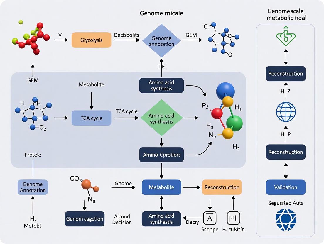
Genome-scale metabolic models (GEMs) represent complex metabolic networks of organisms using stoichiometric matrices to enable systems-level analysis of metabolic functions. These computational tools integrate genomic annotation, biochemical knowledge, and physiological constraints to simulate metabolic capabilities under specific conditions. GEMs have become indispensable in diverse applications ranging from metabolic engineering and drug target identification to understanding microbial ecology and developing live biotherapeutic products. This protocol outlines the core components, stoichiometric principles, and reconstruction methodologies that form the foundation of GEM development and application, providing researchers with a structured framework for model construction and validation.
Genome-scale metabolic models are knowledge-based in silico representations of the metabolic network of an organism, constructed from genomic and biochemical information [1]. They capture a systems-level view of the entirety of metabolic functions within a cell, representing complex interconnections between genes, proteins, reactions, and metabolites [1]. The mathematical foundation of GEMs relies on the stoichiometric matrix (S), where each element Sij represents the stoichiometric coefficient of metabolite i in reaction j [2]. This matrix formulation enables sophisticated constraint-based reconstruction and analysis (COBRA) methods, including Flux Balance Analysis (FBA), to predict metabolic phenotypes and flux distributions under specified conditions [1] [3].
The reconstruction and analysis of GEMs has evolved into a powerful systems biology approach with applications spanning basic understanding of genotype-phenotype relationships to solving biomedical and environmental challenges [1]. Well-curated GEMs exist for over 100 prokaryotes and eukaryotes, providing organized and mathematically tractable representations of these organisms' metabolic networks [1]. The utility of GEMs extends beyond mere metabolic mapping; they provide a framework for integrating species-specific knowledge and complex 'omics data, facilitating the translation of biological hypotheses into testable predictions of metabolic phenotypes [1] [4].
Core Components of GEMs
Fundamental Elements
The reconstruction of genome-scale metabolic models requires the systematic assembly of several core components that collectively represent the metabolic network of an organism.
Table 1: Core Components of Genome-Scale Metabolic Models
| Component | Description | Function in Model |
|---|---|---|
| Genes | DNA sequences encoding metabolic enzymes | Provide genetic basis for metabolic reactions; included via gene-protein-reaction (GPR) associations |
| Proteins | Enzymes catalyzing biochemical reactions | Implement catalytic functions; connect genes to reactions |
| Reactions | Biochemical transformations between metabolites | Form the edges of the metabolic network; include metabolic, transport, and exchange reactions |
| Metabolites | Chemical compounds participating in reactions | Form the nodes of the metabolic network; must be mass and charge-balanced |
| Stoichiometric Matrix | Mathematical representation of reaction stoichiometry | Core mathematical structure; enables constraint-based analysis |
Gene-Protein-Reaction Associations
Gene-protein-reaction (GPR) associations use Boolean expressions to encode the nonlinear mapping between genes and reactions, accounting for metabolic complexities such as multimeric enzymes, multifunctional enzymes, and isoenzymes [1]. These associations define the protein complexes required to catalyze each metabolic reaction and are essential for predicting the metabolic consequences of genetic perturbations. For example, in the S. suis iNX525 model, GPR associations were obtained from reference models of related organisms (Bacillus subtilis, Staphylococcus aureus, and S. pyogenes) using sequence homology criteria (identity ≥ 40% and match lengths ≥ 70%) [2]. Innovative approaches have been developed to represent GPR associations directly within the stoichiometric matrix of GEMs, enabling extension of flux sampling approaches to gene sampling and facilitating quantification of uncertainty [1].
Biomass Composition
The biomass objective function represents the metabolic requirements for cellular growth by accounting for all necessary biomass precursors and their relative contributions. This includes macromolecular components such as proteins, DNA, RNA, lipids, and other cellular constituents. For example, in the S. suis iNX525 model, the biomass composition was adapted from Lactococcus lactis, containing proteins (46%), DNA (2.3%), RNA (10.7%), lipids (3.4%), lipoteichoic acids (8%), peptidoglycan (11.8%), capsular polysaccharides (12%), and cofactors (5.8%) [2]. The specific DNA, RNA, and amino acid compositions were calculated from the genome and protein sequences of S. suis [2].
Table 2: Experimentally Determined Biomass Composition in S. suis iNX525 Model
| Biomass Component | Percentage | Composition Basis |
|---|---|---|
| Proteins | 46% | Calculated from S. suis protein sequences |
| DNA | 2.3% | Calculated from S. suis genome sequence |
| RNA | 10.7% | Calculated from S. suis genome sequence |
| Lipids | 3.4% | Literature values for free fatty acids |
| Lipoteichoic Acids | 8% | Literature values |
| Peptidoglycan | 11.8% | Literature values |
| Capsular Polysaccharides | 12% | Literature values |
| Cofactors | 5.8% | Literature values |
Stoichiometric Principles and Mathematical Foundation
The Stoichiometric Matrix
The core mathematical structure of GEMs is the stoichiometric matrix S, where each element Sij represents the stoichiometric coefficient of metabolite i in reaction j [2]. This matrix formulation captures the topology and stoichiometry of the entire metabolic network, enabling mathematical analysis of metabolic capabilities. The stoichiometric matrix typically has dimensions of m × n, where m is the number of metabolites and n is the number of reactions in the network. For example, the S. suis iNX525 model comprises 708 metabolites and 818 reactions, resulting in a stoichiometric matrix of corresponding dimensions [2].
Flux Balance Analysis
Flux Balance Analysis (FBA) is the primary constraint-based method used to analyze GEMs. FBA operates on the principle of mass conservation in a network under pseudo-steady state conditions, using a stoichiometric matrix and biologically relevant objective functions to determine optimal reaction flux distributions [3]. The mathematical formulation of FBA is represented as:
Maximize Z = cᵀv Subject to: S·v = 0 vmin ≤ v ≤ vmax
Where Z is the objective function (typically biomass production), c is a vector of weights indicating which metabolites contribute to the objective, v is the flux vector through each reaction, S is the stoichiometric matrix, and vmin and vmax are lower and upper bounds on reaction fluxes, respectively [2]. This linear programming formulation allows for prediction of metabolic behavior under specified environmental and genetic conditions.
Model Constraints
The predictive capability of GEMs relies on appropriate constraints that define the biological and environmental limitations on metabolic fluxes:
- Stoichiometric constraints: Enforce mass conservation through the equation S·v = 0, ensuring that metabolite production balances consumption at steady state [2].
- Capacity constraints: Define upper and lower bounds (vmin, vmax) on reaction fluxes based on enzyme capacities or thermodynamic considerations [3].
- Environmental constraints: Limit uptake and secretion rates based on nutrient availability in the growth environment [1] [3].
- Gene knockout constraints: Enable simulation of genetic perturbations by setting fluxes of reactions associated with deleted genes to zero [2].
GEM Reconstruction Protocol
Reconstruction Workflow
The reconstruction of high-quality genome-scale metabolic models follows a systematic protocol encompassing multiple stages of curation and validation.
Detailed Methodologies
Genome Annotation and Draft Reconstruction
The initial step involves identifying genes encoding metabolic enzymes and establishing their functional annotations through homology-based methods [1]. Automated pipelines such as ModelSEED [2], RAVEN [1], AuReMe/Pantograph [1], CarveMe [1], and KBase [1] can generate draft models from annotated genomes. For the S. suis iNX525 model, the genome was initially annotated using RAST and then processed through ModelSEED for automated construction [2]. To improve accuracy, template-based approaches can be employed using previously curated GEMs of closely related organisms as references [2].
Manual Curation and Gap Analysis
Manual curation addresses limitations in automated reconstruction by incorporating organism-specific biochemical knowledge. This process involves:
- Gap analysis: Identifying metabolic gaps that prevent synthesis of essential biomass components using tools like gapAnalysis in the COBRA Toolbox [2].
- Reaction addition: Incorporating missing biochemical reactions based on literature evidence, transporter annotations from databases like TCDB, and new gene functions assigned via BLASTp against UniProtKB/Swiss-Prot [2].
- Mass and charge balancing: Ensuring all reactions are chemically consistent by adding H₂O or H⁺ as needed, verified using checkMassChargeBalance programs [2].
Biomass Formulation
Develop a comprehensive biomass objective function representing the metabolic requirements for cellular growth:
- Determine macromolecular composition percentages from literature or related organisms [2].
- Calculate specific DNA, RNA, and amino acid compositions from genomic and proteomic sequences [2].
- Incorporate experimentally determined compositions for complex components like lipoteichoic acids and capsular polysaccharides [2].
- Formulate the biomass equation as a weighted sum of all biomass precursors.
Model Validation
Validate the metabolic model through multiple approaches:
- Growth simulations: Compare in silico predictions with experimental growth phenotypes under different nutrient conditions [2].
- Gene essentiality: Assess agreement between model-predicted essential genes and experimental mutant screens [2].
- Physiological consistency: Ensure model predictions align with known physiological capabilities of the organism.
For S. suis iNX525, growth assays in chemically defined medium (CDM) with systematic nutrient omissions (leave-one-out experiments) were used to validate model predictions, with growth rates measured by optical density at 600 nm and normalized to growth in complete CDM [2].
Applications of GEMs
Genome-scale metabolic models have diverse applications across biotechnology, biomedicine, and basic research:
- Metabolic Engineering: Identification of gene knockout and overexpression targets for strain optimization [5].
- Drug Target Discovery: Prediction of essential metabolic pathways and reactions for antimicrobial development [2].
- Host-Pathogen Interactions: Analysis of metabolic dependencies during infection [2].
- Microbiome Research: Modeling metabolic interactions in complex microbial communities [3] [4].
- Live Biotherapeutic Products: Guiding the design of microbial consortia for therapeutic applications [4].
In drug discovery, GEMs of pathogens like S. suis enable identification of dual-purpose targets essential for both growth and virulence factor production [2]. For microbiome applications, GEMs facilitate modeling of cross-feeding interactions and nutrient cycling within microbial communities, as demonstrated in sponge holobiont systems [3].
Research Reagent Solutions
Table 3: Essential Research Reagents and Tools for GEM Development
| Reagent/Tool | Function | Application Examples |
|---|---|---|
| COBRA Toolbox | MATLAB toolbox for constraint-based modeling | Model simulation, gap-filling, flux variability analysis [2] |
| ModelSEED | Automated pipeline for draft model reconstruction | Rapid generation of draft models from annotated genomes [2] |
| RAST | Rapid Annotation using Subsystem Technology | Genome annotation for model reconstruction [2] |
| AGORA2 | Resource of curated GEMs for gut microbes | Modeling host-microbiome interactions [4] |
| GUROBI Optimizer | Mathematical optimization solver | FBA simulation for large-scale models [2] |
| MEMOTE | Test suite for model quality assessment | Standardized model evaluation and quality reporting [2] |
| BiGG Database | Curated metabolic database | Reference for biochemical reaction information [1] |
| UniProtKB/Swiss-Prot | Curated protein sequence database | Functional annotation of metabolic enzymes [2] |
Genome-scale metabolic models provide a powerful framework for systems-level analysis of cellular metabolism. The core components—genes, proteins, reactions, metabolites, and their stoichiometric relationships—form a mathematical representation that enables prediction of metabolic phenotypes under various genetic and environmental conditions. The reconstruction protocol outlined here emphasizes the importance of both automated and manual curation processes to develop high-quality models that accurately reflect organismal metabolism. As GEM methodologies continue to advance, they offer increasingly sophisticated approaches for addressing fundamental biological questions and solving applied problems in biotechnology and medicine. Future directions include improved integration of regulatory information, better representation of multi-scale phenomena, and enhanced methods for modeling microbial communities.
The construction of genome-scale metabolic models (GEMs) represents a cornerstone of systems biology, enabling researchers to translate genomic information into predictive computational models of metabolic networks. The journey began with Haemophilus influenzae, the first free-living organism to have its entire genome sequenced and its metabolic network reconstructed [6]. This pioneering work in 1999 established the foundational framework for GEM development, transforming how we investigate the relationship between genotype and phenotype across the tree of life [7]. This application note details the historical progression, core methodologies, and practical protocols in GEM construction, providing a resource for researchers and drug development professionals engaged in metabolic network analysis.
The Foundational Model:Haemophilus influenzae
The first whole-genome metabolic model of H. influenzae strain Rd was a milestone in theoretical biology [6]. This model, reconstructed from the annotated genome sequence, comprised 461 metabolic reactions operating on 367 intracellular metabolites and 84 extracellular metabolites [6]. The reconstruction process involved meticulously mapping genes to proteins and subsequently to biochemical reactions, thereby defining the organism's metabolic genotype.
The initial model was subdivided into six subsystems, and its underlying pathway structure was determined using extreme pathway analysis [6]. This approach, based on stoichiometric, thermodynamic, and system-specific constraints, allowed researchers to address several physiological questions: it helped curate the genome annotation by identifying reactions without functional support, predicted co-regulated gene products, determined minimal substrate requirements for producing essential biomass components, and identified critical gene deletions under different environmental conditions [6]. Under minimal substrate conditions, 11 genes were found to be critical, with six remaining essential even in the more nutrient-rich conditions reflecting the human host environment [6].
Table 1: Key Statistics of the First Genome-Scale Metabolic Model
| Feature | Description |
|---|---|
| Organism | Haemophilus influenzae Rd |
| Publication Year | 1999/2000 [6] [7] |
| Total Reactions | 461 [6] |
| Intracellular Metabolites | 367 [6] |
| Extracellular Metabolites | 84 [6] |
| Primary Analysis Method | Extreme Pathway Analysis [6] |
Expansion and Evolution of GEM Construction
Since the inception of the H. influenzae model, the field of GEM construction has experienced exponential growth. As of 2022, GEMs have been constructed for 5,897 bacteria, alongside numerous models for eukaryotic organisms [7]. Key model organisms such as Escherichia coli, Saccharomyces cerevisiae, and Bacillus subtilis have seen multiple iterative updates of their models, enhancing the coverage of gene-protein-reaction associations and improving predictive accuracy [7].
The fundamental principle of GEMs is the transformation of cellular growth and metabolism into a mathematical framework based on a stoichiometric matrix, which is solved for an optimal solution at a steady state [7]. The primary algorithm for simulating phenotypic states from these models is Flux Balance Analysis (FBA), which computes the flow of metabolites through the metabolic network, enabling predictions of growth rates or metabolite production [7].
Table 2: Evolution of GEMs for Key Model Organisms
| Organism | Number of Reported GEMs | Notable Advancements |
|---|---|---|
| Escherichia coli | 13 | Development of Metabolism-Expression (ME) models that reconstruct complete transcription and translation pathways [7]. |
| Saccharomyces cerevisiae | 13 | Latest model (Yeast8) can dissect metabolic mechanisms at multiscale levels [7]. |
| Bacillus subtilis | 7 | Integration of enzymatic data for central carbon metabolism to guide strain engineering [7]. |
Advanced Methodologies: From Constraint-Based to Multiscale Models
Basic GEMs have evolved into sophisticated multiscale models that integrate additional biological layers to more accurately simulate in vivo conditions. The limitation of traditional GEMs, which primarily capture gene-protein-reaction relationships, has prompted the development of models that incorporate various constraints and omics data.
Constraint-Based Modeling
To enhance the predictive power of GEMs, several constraint-based approaches have been developed:
- Thermodynamic Constraint Models: These models incorporate the directionality and Gibbs free energy of metabolic reactions to eliminate thermodynamically infeasible pathways. Key algorithms include Thermodynamically based Metabolic Flux Analysis (TMFA) and network-embedded thermodynamic analysis [7].
- Enzymatic Constraint Models: Frameworks like GECKO integrate enzyme concentration data and catalytic constants into the models, accounting for the proteomic cost of metabolic fluxes [7].
- Kinetic Constraint Models: Approaches such as ORACLE and Ensemble Modeling introduce kinetic parameters to evaluate the dynamic properties of metabolic systems, moving beyond steady-state assumptions [7].
Multi-Omics Integration
The development of high-throughput technologies has enabled the integration of multi-omics data (e.g., transcriptomics, proteomics) directly into GEMs. Algorithmic frameworks such as iMAT, MADE, and GIM3E leverage these data to create context-specific models, improving their biological relevance and predictive accuracy for particular conditions [7]. Furthermore, tools like TIGER and FlexFlux integrate transcriptional regulatory networks with GEMs, allowing for the simulation of complex regulatory-metabolic interactions [7].
Essential Protocols and Workflows
Workflow for GEM Construction and Analysis
The following diagram outlines the generalized workflow for constructing and analyzing genome-scale metabolic models, from genomic data to model validation and application.
Protocol: Tn-seq Mutant Library Generation forHaemophilus influenzae
This protocol details the generation of a transposon sequencing (Tn-seq) mutant library, a genome-wide screen used to identify conditionally essential bacterial genes, such as those involved in virulence [8]. The following workflow summarizes the key stages of this protocol.
Part I: Generation of Mutant Library [8]
Transposition Reaction
- Prepare a fresh 6x transposition buffer containing glycerol, DTT, Hepes, BSA, NaCl, and MgCl₂.
- Combine 3.3 µL of 6x Transposition Buffer with 0.5-1.0 µg recipient DNA (e.g., chromosomal DNA of the target strain), 0.5-1.0 µg donor DNA containing the mariner transposon with an MmeI restriction site, 1 µL recombinant Himar1 transposase, and sterile dH₂O to a total volume of 20 µL.
- Mix and incubate for 4 hours at 30°C.
- Inactivate the transposase by heating at 75°C for 10 minutes.
- Precipitate the DNA using sodium acetate, glycogen, and absolute ethanol.
Repair of Transposition Reaction
- Resuspend the pellet and add T4 DNA polymerase Reaction Buffer, BSA, dNTP mix, and T4 DNA polymerase.
- Incubate for 30 minutes at 16°C to repair the transposed DNA.
- Inactivate the polymerase at 75°C for 10 minutes and precipitate the DNA again.
Transformation and Library Selection
- Transform the repaired transposition reaction into naturally competent non-typeable H. influenzae.
- Plate the transformation on selective supplemented Brain Heart Infusion (sBHI) agar plates.
- Harvest the mutants by adding PBS, scrape the plates, and pool all colonies. The resulting library can be used for functional screens under challenge conditions (e.g., survival in environmental air).
Part II: Mutant Library Readout and Data Analysis [8]
Genomic DNA Preparation and Adapter Ligation
- Extract genomic DNA from the mutant library before and after screening using a Qiagen Genomic-tip.
- Digest the genomic DNA with MmeI, which cuts at the specific site engineered within the transposon.
- Ligate sequence adapters to the digested fragments.
PCR Amplification and Sequencing
- Amplify the fragments using primers complementary to the ligated adapters.
- The resulting PCR product is sequenced using a high-throughput platform like Illumina MiSeq.
Data Analysis
- The sequencing reads are mapped to the genome to identify transposon insertion sites and their abundance.
- Use web-based analysis software such as ESSENTIALS to identify genes essential for growth under the tested condition by comparing insertion abundances between control and challenge libraries.
Research Reagent Solutions
Table 3: Key Reagents for Tn-seq and Genomic Analysis
| Reagent/Kit | Function | Example Use Case |
|---|---|---|
| Himar1 Mariner Transposase | Catalyzes random insertion of transposon into TA dinucleotide sites in the genome. | Essential for in vitro transposition reaction to generate random mutant library [8]. |
| MmeI Restriction Enzyme | Cuts DNA at a specific site (TCCRAC) 20/18 bases away from its recognition site. | Used to digest genomic DNA, generating a short fragment that includes the transposon end and adjacent genomic sequence for sequencing [8]. |
| T4 DNA Polymerase | Possesses DNA polymerase and single-stranded exonuclease activities. | Repairs the transposed DNA after the in vitro transposition reaction [8]. |
| Qiagen Genomic-tip Columns | Silica-gel membrane-based technology for purification of high-molecular-weight genomic DNA. | Essential for obtaining high-quality genomic DNA required for the Tn-seq library preparation [8]. |
| ESSENTIALS Software | Web-based tool for the analysis of Tn-seq data. | Identifies conditionally essential genes by statistically comparing transposon insertion frequencies between libraries [8]. |
The historical trajectory from the first Haemophilus influenzae GEM to the thousands of models in existence today underscores the transformative impact of this methodology on systems biology and metabolic engineering. The initial reconstruction, containing hundreds of reactions, has evolved into multiscale models that integrate thermodynamic, enzymatic, and regulatory constraints. Supported by robust experimental protocols like Tn-seq and powerful computational algorithms, GEMs provide an indispensable framework for elucidating genotype-phenotype relationships. As the field progresses with the integration of machine learning and more complex multi-omics data, GEMs will continue to be pivotal in advancing scientific discovery and streamlining drug and bioproduction development.
Genome-scale metabolic models (GEMs) are computational representations of the metabolic network of an organism, and their core component is the set of Gene-Protein-Reaction (GPR) associations [9]. These logical rules mathematically define the connection between an organism's genes and its metabolic capabilities by explicitly describing how genes encode proteins (enzymes) that catalyze specific biochemical reactions [10]. GPR rules use Boolean logic (AND and OR operators) to represent the genetic basis of metabolism: the AND operator joins genes encoding different subunits of the same enzyme complex, while the OR operator joins genes encoding distinct isozymes that can catalyze the same reaction [10].
The reconstruction of accurate GPRs is therefore a fundamental step in building high-quality GEMs, transforming an abstract network of biochemical reactions into a genotype-prediction model capable of simulating the metabolic consequences of genetic perturbations [11]. This protocol details the methods for establishing these critical genetic links, enabling researchers to move from a genome sequence to a functional, predictive metabolic model.
Key Concepts and Quantitative Landscape
A survey of current resources reveals that GEMs have been reconstructed for thousands of organisms. The table below summarizes the current status of manually and automatically reconstructed GEMs across different domains of life [9].
Table 1: Current Status of Reconstructed Genome-Scale Metabolic Models (as of February 2019)
| Domain of Life | Total GEMs | Manually Reconstructed | Example Organisms |
|---|---|---|---|
| Bacteria | 5,897 | 113 | Escherichia coli, Bacillus subtilis, Mycobacterium tuberculosis |
| Archaea | 127 | 10 | Methanosarcina acetivorans |
| Eukaryotes | 215 | 60 | Saccharomyces cerevisiae, Homo sapiens |
The complexity of GPR associations within a model can be statistically analyzed. In the E. coli iAF1260 model, for instance [11]:
- Over 16% of enzymes are protein complexes (requiring AND logic in GPRs).
- Approximately 31% of metabolic reactions are catalyzed by multiple isozymes (requiring OR logic in GPRs).
- More than 72% of reactions are catalyzed by at least one promiscuous enzyme.
This logical structure of GPR associations can be visualized as a network, as shown in the diagram below.
Diagram 1: Logic of GPR associations. AND operators join genes encoding subunits of a complex. OR operators join genes encoding isozymes.
Protocols for GPR Reconstruction
Protocol 1: Manual Reconstruction and Curation of GPRs
Manual curation remains the gold standard for developing high-quality, reference-grade GEMs. This protocol is essential for model organisms or when high predictive accuracy is required.
Table 2: Key Data Sources for Manual GPR Reconstruction
| Data Source | Type of Information | Role in GPR Reconstruction |
|---|---|---|
| Genome Annotation | Gene identities and locations | Provides the initial list of metabolic genes [10]. |
| UniProt | Protein functional data, complex subunits | Provides evidence for protein complexes and isoform data [10] [12]. |
| KEGG | Pathway maps, enzyme nomenclature | Validates reaction assignments and fills pathway gaps [10] [13]. |
| MetaCyc | Curated biochemical pathways | Provides experimentally verified metabolic information [10]. |
| Complex Portal | Protein-protein interactions, complexes | Critical for defining AND relationships in GPR rules [10]. |
| Scientific Literature | Experimental biochemical evidence | Provides direct validation for GPR associations [10]. |
Step-by-Step Procedure:
- Gene List Compilation: Generate a comprehensive list of metabolic genes from the organism's genome annotation file (e.g., GFF format) or databases like NCBI.
- Reaction Assignment: Assign metabolic reactions to each gene product based on enzyme commission (EC) numbers and homology to well-annotated genes in reference databases (KEGG, MetaCyc).
- Protein Complex and Isozyme Resolution: For each reaction, consult UniProt and the Complex Portal to determine:
- If the reaction is catalyzed by a protein complex (requires AND logic between subunit genes).
- If multiple distinct proteins or complexes can catalyze the reaction (requires OR logic between genes/complexes).
- Boolean Rule Formulation: Write the GPR rule in Boolean logic format. For example:
- A homomeric enzyme:
Gene_A - A heteromeric complex:
Gene_A and Gene_B - Multiple isozymes:
Gene_C or Gene_D - A complex with isozymes:
(Gene_A and Gene_B) or (Gene_C and Gene_D)
- A homomeric enzyme:
- Experimental Validation: Use phenotypic data (e.g., growth on different carbon sources) and gene essentiality data to test and refine the GPR rules. A correctly formulated GPR should accurately predict the growth outcome of gene knockout experiments [9] [13].
Protocol 2: Automated Reconstruction Using GPRuler
For high-throughput reconstruction or for non-model organisms, automated tools are highly efficient. GPRuler is an open-source Python framework designed to fully automate GPR reconstruction [10].
Workflow: The GPRuler pipeline automates the information retrieval and logic assembly steps of GPR creation, as illustrated below.
Diagram 2: GPRuler automated reconstruction workflow.
Step-by-Step Procedure:
- Input: Provide the tool with either just the name of the target organism or an existing draft metabolic model (in SBML format) that lacks GPR associations.
- Execution: Run the GPRuler pipeline. The tool will automatically:
- Query its integrated biological databases (MetaCyc, KEGG, UniProt, Complex Portal, etc.) to retrieve relevant gene, protein, and complex information for the target organism.
- Process this information to identify protein complexes (requiring AND operators) and isozymes (requiring OR operators).
- Assemble the correct Boolean GPR rule for each metabolic reaction.
- Output: Obtain a curated SBML model containing the GPR rules. The tool has demonstrated high accuracy in reproducing GPR rules in benchmark models for Homo sapiens and Saccharomyces cerevisiae [10].
Advanced Applications and Integration
Stoichiometric Representation for Gene-Level Phenotype Prediction
A advanced use of GPRs is their transformation into a stoichiometric representation that can be integrated directly into the model's stoichiometric matrix [11]. This method explicitly represents the enzyme (or subunit) encoded by each gene as a pseudo-metabolite in the model. This transformation enables constraint-based analysis to predict phenotypes directly at the gene level, overcoming limitations of traditional Boolean interpretation.
Procedure:
- Model Transformation: Decompose reversible reactions and reactions catalyzed by multiple isozymes into individual, irreversible reactions.
- Introduce Enzyme Usage Variables: For each gene, add a new "enzyme usage" reaction (
u_gene) that accounts for the total flux carried by the respective enzyme or subunit. - Reformulate Constraints: Incorporate these new variables and pseudo-species into the stoichiometric matrix, creating an extended model.
- Perform Gene-Level Analysis: Apply standard constraint-based methods (e.g., FBA, pFBA) to the extended model. The solution vector will now include fluxes for the enzyme usage variables, providing a direct link between gene expression and metabolic flux [11].
Integration with Omics Data Using ICON-GEMs
GPRs are essential for integrating transcriptomic data into GEMs. The ICON-GEMs method is an innovative approach that integrates gene co-expression networks with GEMs to improve the prediction of condition-specific flux distributions [14].
Step-by-Step Protocol:
- Data Preparation: Process gene expression profiles (e.g., RNA-seq data) for the condition of interest, handling missing values and outliers.
- Co-expression Network Construction: Calculate pairwise Pearson correlation coefficients between all genes and transform them into a binary adjacency matrix using a defined threshold.
- Model Constraining: Use the E-flux method to set the upper bounds for reaction fluxes based on the expression levels of the associated genes, as defined by the GPR rules.
- Quadratic Programming Optimization: Solve the ICON-GEMs formulation, which maximizes the alignment between pairs of reaction fluxes and the correlation of their corresponding genes in the co-expression network. The objective function is:
Maximize Σ (qi * qj) for all reaction pairs (i, j) whose genes are linked in the co-expression network.
Where
qrepresents transformed reaction flux values, subject to the standard stoichiometric and capacity constraints [14].
Validation and Experimental Design
Protocol for Validating GPRs via Phenotypic Assays
Computationally derived GPR rules must be validated experimentally. The most common method is to compare in silico predictions of gene essentiality and substrate utilization with in vivo experimental results.
Experimental Design:
- In silico Prediction:
- Gene Essentiality: For each gene in the model, simulate a knockout by setting its activity to
FALSEin the GPR rule. Predict growth under a defined condition (e.g., minimal glucose medium). A gene is predicted to be essential if the simulated growth rate is zero. - Substrate Utilization: Simulate growth on a panel of different carbon or nitrogen sources.
- Gene Essentiality: For each gene in the model, simulate a knockout by setting its activity to
- In vivo Experimentation:
- Gene Knockouts: Create a library of single-gene knockout strains.
- Phenotypic Microarray: Use high-throughput growth assays (e.g., in Biolog plates) to experimentally determine the essentiality of each gene and the organism's ability to utilize different substrates.
- Validation and Model Refinement: Calculate the prediction accuracy by comparing the computational and experimental results. Discrepancies often point to incorrect GPR rules, missing transport reactions, or gaps in the metabolic network, guiding further manual curation [13].
Table 3: Example Validation Metrics for the S. radiopugnans iZDZ767 Model [13]
| Validation Type | Condition/Genes Tested | Prediction Accuracy |
|---|---|---|
| Carbon Source Utilization | 28 different carbon sources | 82.1% (23/28) |
| Nitrogen Source Utilization | 6 different nitrogen sources | 83.3% (5/6) |
| Gene Essentiality | Single gene knockouts | 97.6% |
The Scientist's Toolkit
Table 4: Essential Research Reagents and Computational Tools
| Item / Tool Name | Type | Function in GPR Research |
|---|---|---|
| GPRuler | Software Tool | Fully automated reconstruction of GPR rules from an organism name or draft model [10]. |
| COBRA Toolbox | Software Suite (MATLAB) | Industry-standard platform for constraint-based modeling, including simulation and analysis of GPR-enabled models [13]. |
| UniProt Knowledgebase | Database | Provides critical information on protein complexes and isoforms, essential for defining AND/OR logic [10] [12]. |
| Complex Portal | Database | A key resource for protein-protein interaction data and stoichiometry of complexes [10]. |
| Merlin | Software Tool | An integrated platform for genome-scale metabolic reconstruction that includes GPR assignment features [10]. |
| ModelSEED / RAVEN | Software Toolboxes | Assist in semi-automated draft model reconstructions, including the assignment of GPR associations [10] [13]. |
| Phenotypic Microarray Plates | Laboratory Consumable | High-throughput experimental validation of growth phenotypes predicted by the model [13]. |
| pyTARG Library | Software Tool (Python) | A custom library for integrating RNA-seq data into GEMs to quantify drug effects, relying on GPR rules [15]. |
Genome-scale metabolic models (GEMs) are computational frameworks that systematically simulate an organism's metabolic network by integrating gene-protein-reaction (GPR) associations, stoichiometry, and compartmentalization data [16]. For model organisms such as Escherichia coli, Saccharomyces cerevisiae, and Mycobacterium tuberculosis, the development of multiple, iterative GEMs has created a need for systematic benchmarking to guide researchers in model selection for specific applications such as metabolic engineering, drug target identification, and systems biology studies [16] [17]. This application note provides a structured comparison of key organism-specific GEMs, detailed experimental protocols for their evaluation, and essential reagent solutions to facilitate their use in research and drug development contexts.
The continuous refinement of GEMs for key organisms has resulted in models of varying scope, from comprehensive genome-scale reconstructions to streamlined, curated models optimized for specific analysis types.
1Saccharomyces cerevisiaeModels
The development of GEMs for S. cerevisiae began in 2003 with the iFF708 model and has progressed through a series of consensus models [16]. The trajectory has advanced from Yeast1 to the latest iterations, Yeast8 and Yeast9.
Table 1: Key Genome-Scale Metabolic Models for S. cerevisiae
| Model Name | Key Features | Reactions | Genes | Primary Applications |
|---|---|---|---|---|
| Yeast8 | Base for yETFL; includes SLIME reactions; updated GPR associations [16] [18] | 3,991 | 1,149 | Generation of advanced multi-scale models; template for strain-specific models [16] |
| Yeast9 | Refined mass/charge balances; thermodynamic parameters; integrated single-cell transcriptomics [16] | Information not in search results | Information not in search results | Analysis of yeast adaptation to stress (e.g., high osmotic pressure) [16] |
| yETFL | Integrates metabolic, protein, and RNA synthesis; incorporates thermodynamic constraints & enzyme kinetics [18] | Information not in search results | 1,393 (1,149 metabolic + 244 expression system) | Prediction of growth rates, essential genes, and overflow metabolism under expression constraints [18] |
2Mycobacterium tuberculosisModels
Multiple GEMs have been constructed for M. tuberculosis strain H37Rv, derived primarily from two early reconstructions: GSMN-TB and iNJ661 [17]. A systematic evaluation of eight models identified two as top performers.
Table 2: Benchmarking of Select M. tuberculosis H37Rv GEMs
| Model Name | Precursor/Origin | Key Strengths | Notable Limitations |
|---|---|---|---|
| iEK1011 | Consolidated model using BiGG database standardization [17] | High gene similarity (>60%) with all other models; good performance in gene essentiality prediction [17] | Performance details not in search results |
| sMtb2018 | Combination of three previous models [17] | High gene similarity with other models; designed for modeling metabolism inside macrophages [17] | Performance details not in search results |
| iOSDD890 | Curated update of iNJ661 [17] | High coverage of nitrogen, propionate, and pyrimidine metabolism [17] | Lacks β-oxidation pathways; cannot simulate growth on fatty acids [17] |
3Escherichia coliModels
The modeling landscape for E. coli includes both genome-scale and focused, manually-curated models designed for specific analytical tasks.
Table 3: Representative E. coli K-12 MG1655 Metabolic Models
| Model Name | Scale | Reactions | Genes | Purpose and Utility |
|---|---|---|---|---|
| iML1515 | Genome-Scale | 2,712 | 1,515 | Comprehensive metabolic network; template for smaller models [19] |
| iCH360 | Medium-Scale ("Goldilocks") | 323 | 360 | Manually curated model of core energy and biosynthetic metabolism; avoids unphysiological predictions [19] |
| ECC2 | Medium-Scale | Information not in search results | Information not in search results | Algorithmically reduced model; retains ability to produce biomass precursors [19] |
Experimental Protocols for Model Evaluation and Application
Protocol: Systematic Evaluation of Multiple GEMs
This protocol is adapted from the methodology used to benchmark M. tuberculosis GEMs [17] and can be applied to evaluate models for any organism.
1. Descriptive Model Evaluation
- Objective: Compare basic structural properties and network connectivity.
- Procedure:
- Calculate and compare the number of reactions, metabolites, and genes for each model.
- Perform a set theory-based analysis to identify the core set of genes common to all models and strain-specific accessory genes [17].
- Identify and map blocked reactions (reactions that cannot carry flux under any condition) and gaps in the metabolic network.
- Output: A quantitative inventory of model components and coverage of essential pathways.
2. Assessment of Thermodynamic Feasibility
- Objective: Identify thermodynamically infeasible cycles that can lead to unrealistic flux predictions.
- Procedure:
- Output: A list of infeasible cycles and a thermodynamically curated model.
3. Phenotypic Prediction Accuracy
- Objective: Test the model's ability to recapitulate known experimental phenotypes.
- Procedure:
- Growth Simulation: Use Flux Balance Analysis (FBA) to predict growth capabilities on different carbon and nitrogen sources (e.g., glucose, cholesterol for Mtb) [17].
- Gene Essentiality Prediction: Simulate single-gene knockout strains and compare the predictions of essential/non-essential genes against experimental gene essentiality data [17].
- Flux Variability Analysis (FVA): Determine the range of possible fluxes for each reaction to assess network flexibility [17].
Protocol: Constructing an Expression-Mechanics Model from a GEM
This protocol outlines the steps for building a multi-scale model like yETFL, which integrates metabolism with expression constraints [18].
1. Thermodynamic Curation of the Base GEM
- Objective: Establish a thermodynamically consistent foundation.
- Procedure:
- Obtain standard Gibbs free energies of formation (ΔfG'°) for metabolites using group contribution methods [18].
- For reactions in aqueous environments, calculate the Gibbs free energy of reaction (ΔrG'°).
- Constrain reaction directions in the model to be consistent with their calculated ΔrG'° values.
2. Integration of Enzyme Kinetics and Catalytic Constraints
- Objective: Incorporate proteomic limitations.
- Procedure:
- Compile enzyme turnover numbers (kcat) from databases and literature. Use median kcat values for enzymes with unknown kinetics [18].
- Formulate catalytic constraints that couple metabolic flux through a reaction to the abundance and catalytic capacity of its enzyme.
- Model the synthesis of enzyme complexes from their constituent peptides.
3. Implementation of the Expression Machinery
- Objective: Account for the biosynthetic costs of proteins and RNAs.
- Procedure:
- For eukaryotes like S. cerevisiae, include separate ribosomes and RNA polymerases for the nucleus and mitochondria [18].
- Define constraints that represent the cellular capacity for transcription and translation.
- Discretize the growth range (e.g., [0, μ_max]) into multiple bins to linearize the problem and enable solution via mixed-integer linear programming (MILP) [18].
Table 4: Key Reagent Solutions for GEM Construction and Analysis
| Reagent/Resource | Function | Example Tools/Databases |
|---|---|---|
| Reconstruction Toolboxes | Automated draft model generation from genomic data | RAVEN Toolbox [16], CarveFungi [16] |
| Constraint-Based Analysis Suites | Simulation and analysis of GEMs (FBA, FVA, etc.) | COBRApy [19] |
| Thermodynamic Databases | Estimation of Gibbs free energy for metabolites and reactions | Group Contribution Method [18] |
| Enzyme Kinetics Databases | Provision of enzyme turnover numbers (kcat) | Published literature and specialized databases [18] |
| Visualization Platforms | Creation of custom metabolic maps for model visualization | Escher [19] |
| Standardized Model Databases | Access to curated models and reactions using standardized nomenclature | BiGG Models [17] |
Workflow and Relationship Diagrams
GEM Evaluation and Selection Workflow
The following diagram outlines the logical process for systematically evaluating and selecting a GEM for a research project, based on the benchmarking study of M. tuberculosis models [17].
GEM Selection Workflow: This chart outlines the systematic process for evaluating and selecting a genome-scale metabolic model, from initial assembly to final application.
Multi-Scale Model Development Process
This diagram illustrates the process of enhancing a standard GEM into a multi-scale model by integrating additional layers of biological constraints, as demonstrated by the development of yETFL [18].
Multi-Scale Model Development: This flowchart shows the sequential layering of thermodynamic, enzymatic, and expression constraints onto a base GEM to create a more predictive multi-scale model.
Flux Balance Analysis (FBA) is a cornerstone mathematical approach within the constraint-based modeling framework for analyzing the flow of metabolites through metabolic networks [20]. As a computational method, it enables the prediction of steady-state metabolic fluxes in genome-scale metabolic models (GEMs), which represent the entire metabolic repertoire of an organism based on its genomic annotation [9]. FBA has gained prominence as a powerful systems biology tool because it can simulate metabolism without requiring extensive kinetic parameter data, instead relying on stoichiometric constraints and optimization principles to predict cellular behavior [20] [21]. This capability makes FBA particularly valuable for harnessing the knowledge encoded in the growing number of GEMs, with models now available for thousands of organisms across bacteria, archaea, and eukarya [9].
The fundamental value of FBA lies in its ability to transform static genome-scale metabolic reconstructions into dynamic models that can predict phenotypic outcomes from genotypic information [22]. By calculating the flow of metabolites through metabolic networks, FBA enables researchers to predict critical cellular phenotypes such as growth rates, nutrient uptake rates, by-product secretion, and the metabolic consequences of genetic modifications [20] [23]. This predictive capacity has made FBA an indispensable tool in both basic research and applied biotechnology, supporting applications ranging from microbial strain engineering for industrial biotechnology to identifying novel drug targets in pathogens [21] [9] [24].
Mathematical Foundations
The mathematical framework of FBA is built upon stoichiometric constraints, mass-balance equations, and optimization theory [20]. This foundation allows FBA to systematically analyze metabolic capabilities without detailed kinetic information, instead focusing on the network structure and mass conservation principles.
Stoichiometric Matrix Representation
The core mathematical representation in FBA is the stoichiometric matrix S, of size m × n, where m represents the number of metabolites and n the number of reactions in the metabolic network [20]. Each element Sᵢⱼ of this matrix contains the stoichiometric coefficient of metabolite i in reaction j. By convention, negative coefficients indicate metabolite consumption, positive coefficients indicate metabolite production, and zero values indicate no participation [20]. This matrix formulation comprehensively captures the structure of the metabolic network and serves as the foundation for all subsequent constraint-based analyses.
Mass Balance Constraints
The fundamental constraint in FBA is the steady-state mass balance assumption, which requires that the concentration of internal metabolites remains constant over time [20] [21]. This is mathematically represented by the equation:
S · v = 0
where v is the n-dimensional vector of metabolic reaction fluxes [20]. This equation ensures that for each metabolite in the network, the total flux producing the metabolite equals the total flux consuming it, thus maintaining constant metabolite concentrations at steady state [21]. For realistic large-scale metabolic models where the number of reactions typically exceeds the number of metabolites (n > m), this system of equations is underdetermined, meaning there is no unique solution [20].
Flux Constraints and Boundary Conditions
To make the underdetermined system tractable, FBA incorporates additional constraints on reaction fluxes:
vₗ ≤ v ≤ vᵤ
where vₗ and vᵤ represent the lower and upper bounds for each reaction flux, respectively [20]. These bounds incorporate known physiological constraints, such as:
- Irreversible reactions (v ≥ 0)
- Measured substrate uptake rates
- Thermodynamic and enzyme capacity constraints
- Environmental conditions (e.g., oxygen availability)
Objective Function and Linear Programming
FBA identifies a particular flux distribution from the possible solution space by optimizing a biologically relevant objective function [20]. The general formulation becomes:
Maximize Z = cᵀv Subject to: S · v = 0 vₗ ≤ v ≤ vᵤ
where c is a vector of weights indicating how much each reaction contributes to the objective function [20]. In practice, when maximizing a single reaction (such as biomass production), c is typically a vector of zeros with a value of 1 at the position of the reaction of interest [20]. This optimization problem is solved using linear programming, which efficiently identifies optimal solutions even for large-scale metabolic networks [20] [21].
Table 1: Key Components of the FBA Mathematical Framework
| Component | Symbol | Description | Role in FBA |
|---|---|---|---|
| Stoichiometric Matrix | S | m × n matrix of stoichiometric coefficients | Defines network structure and mass balance constraints |
| Flux Vector | v | n-dimensional vector of reaction fluxes | Variables to be solved representing metabolic reaction rates |
| Mass Balance | S·v = 0 | System of linear equations | Ensures metabolic steady state |
| Flux Bounds | vₗ, vᵤ | Lower and upper flux constraints | Incorporates physiological and environmental limitations |
| Objective Function | Z = cᵀv | Linear combination of fluxes | Defines biological objective to be optimized |
Computational Implementation
Core Protocol for Flux Balance Analysis
The standard workflow for implementing FBA consists of five key steps that transform a metabolic reconstruction into a predictive model:
Step 1: Model Construction and Curation
- Compile a stoichiometrically balanced metabolic network reconstruction including all known metabolic reactions, metabolites, and gene-protein-reaction (GPR) associations [9]
- Verify mass and charge balance for all reactions
- Define metabolic compartments (for eukaryotic organisms) and transport reactions
Step 2: Define Environmental Constraints
- Specify nutrient availability in the growth medium by setting upper bounds on exchange reactions [20]
- Constrain oxygen uptake rates for aerobic/anaerobic simulations [20]
- Set constraints on by-product secretion based on experimental measurements
Step 3: Formulate the Objective Function
- Select an appropriate biological objective based on the research question [20]
- Common objectives include:
- Biomass maximization (for growth prediction)
- ATP production (for energy metabolism studies)
- Product synthesis (for metabolic engineering)
- Nutrient uptake optimization
Step 4: Solve the Linear Programming Problem
- Apply linear programming algorithms to maximize/minimize the objective function [20]
- Verify solution feasibility and optimality
- Extract the flux distribution vector v corresponding to the optimal solution
Step 5: Validate and Interpret Results
- Compare predictions with experimental data (growth rates, substrate uptake, by-product secretion) [20]
- Perform sensitivity analysis to assess robustness of predictions
- Identify key metabolic pathways contributing to the objective
Advanced FBA Variants
Several extended FBA methodologies have been developed to address specific biological questions and overcome limitations of the standard approach:
Metabolite Dilution FBA (MD-FBA) MD-FBA accounts for growth-associated dilution of all intermediate metabolites, not just those included in the biomass reaction [23]. This is particularly important for metabolites participating in catalytic cycles, such as metabolic co-factors, and improves predictions of gene essentiality and growth rates under different conditions [23]. MD-FBA is formulated as a mixed-integer linear programming (MILP) problem to handle the discrete decisions involved in accounting for dilution of all produced metabolites.
Dynamic FBA (dFBA) dFBA extends the steady-state approach to dynamic conditions by solving a series of FBA problems over time, incorporating changing extracellular metabolite concentrations and using the predicted growth rates to update these concentrations at each time step [22].
Regulatory FBA (rFBA) rFBA incorporates transcriptional regulatory constraints by integrating Boolean logic rules based on gene expression states, thereby constraining reaction activity based on regulatory information in addition to stoichiometric constraints [25].
Flux Variability Analysis (FVA) FVA identifies the range of possible fluxes for each reaction while maintaining optimal or near-optimal objective function values, addressing the issue of multiple optimal solutions in FBA [20].
Table 2: Computational Tools for Flux Balance Analysis
| Tool Name | Primary Function | Key Features | Applications |
|---|---|---|---|
| COBRA Toolbox [20] | MATLAB-based suite for constraint-based analysis | Comprehensive implementation of FBA and related methods; support for SBML models | General metabolic modeling, gene essentiality analysis |
| ModelSEED [26] | Web-based model reconstruction and analysis | Automated pipeline for generating GEMs from genome annotations | Rapid model construction, gap-filling |
| CarveMe [26] | Automated model reconstruction | Top-down approach using core metabolic model; diamond-based gap-filling | High-throughput model building |
| RAVEN [26] | MATLAB-based reconstruction and analysis | Integration with KEGG and MetaCyc; manual curation interface | Eukaryotic model reconstruction, yeast metabolism |
| OptFlux [21] | Metabolic engineering platform | Strain design algorithms; visualization capabilities | Metabolic engineering, knockout prediction |
Applications in Metabolic Research
Prediction of Growth Phenotypes
FBA enables accurate prediction of microbial growth rates under various genetic and environmental conditions [20]. For example, FBA predictions of E. coli growth under aerobic (1.65 hr⁻¹) and anaerobic (0.47 hr⁻¹) conditions with glucose limitation have shown strong agreement with experimental measurements [20]. The protocol for growth prediction involves:
- Constraining the glucose uptake rate to a physiologically realistic level (e.g., 18.5 mmol gDW⁻¹ hr⁻¹)
- Setting appropriate oxygen uptake constraints (high for aerobic, zero for anaerobic)
- Maximizing the flux through the biomass objective function
- Comparing the predicted growth rate with experimental data
Gene Essentiality and Knockout Analysis
FBA can systematically identify essential metabolic genes by simulating the effect of gene deletions [20] [21]. The standard protocol involves:
- For each gene in the model, constrain the flux through all associated reactions to zero based on GPR rules
- Re-optimize the biomass objective function
- Classify genes as essential if the predicted growth rate falls below a threshold (typically 1-5% of wild-type)
- Validate predictions against experimental knockout data
This approach has been extended to double gene knockout analysis, enabling identification of synthetic lethal interactions [20]. For example, FBA has been used to explore all pairwise combinations of 136 E. coli genes to identify double knockouts that are lethal despite single knockouts being viable [20].
Metabolic Engineering and Strain Design
FBA supports rational design of microbial strains for industrial biotechnology by predicting genetic modifications that enhance product yields [21] [9]. Algorithms such as OptKnock use FBA to identify gene deletion strategies that couple desired product formation with growth [20] [21]. The implementation protocol includes:
- Formulating a bi-level optimization problem that maximizes product formation while maintaining growth
- Using mixed-integer linear programming to identify optimal gene knockouts
- Validating predicted strain designs experimentally
- Applications include production of biofuels, organic acids, and pharmaceutical precursors
Host-Microbe Interactions
FBA enables modeling of metabolic interactions between hosts and their associated microbiota [26]. The protocol for constructing host-microbe metabolic models involves:
- Reconstructing or retrieving individual GEMs for host and microbial species
- Integrating models into a unified framework using standardized metabolite nomenclature
- Defining metabolite exchange between host and microbial compartments
- Simulating the integrated system to predict metabolic cross-feeding and dependencies
This approach has been applied to study host-pathogen interactions, including Mycobacterium tuberculosis in alveolar macrophages [9], and to understand the role of gut microbiota in human health and disease [26].
Visualization of FBA Workflow
Diagram 1: FBA Workflow from Reconstruction to Prediction
Research Reagent Solutions
Table 3: Essential Resources for FBA Implementation
| Resource Type | Specific Tools/Databases | Function in FBA Research |
|---|---|---|
| Model Databases | BiGG [26], AGORA [26], MetaNetX [26] | Provide curated metabolic models for various organisms |
| Reconstruction Tools | ModelSEED [26], CarveMe [26], RAVEN [26] | Automate generation of draft GEMs from genomic data |
| Simulation Software | COBRA Toolbox [20], OptFlux [21], COBRApy | Implement FBA algorithms and related methods |
| Linear Programming Solvers | Gurobi, CPLEX, GLPK [26] | Provide optimization algorithms for solving LP problems |
| Model Standards | SBML [20], SMBL-ML | Enable model exchange and interoperability between tools |
| Organism-Specific Models | iML1515 (E. coli) [9], Yeast8 (S. cerevisiae) [9], Recon3D (Human) [26] | Provide high-quality reference models for key organisms |
Protocol for Gene Essentiality Prediction
The following detailed protocol outlines the steps for predicting gene essentiality using FBA, a fundamental application in metabolic network analysis:
Step 1: Model Preparation
- Load the genome-scale metabolic model (in SBML format) using the
readCbModelfunction in the COBRA Toolbox [20] - Verify model quality by checking for mass and charge balance violations
- Set baseline constraints to define the simulated growth condition:
- Carbon source uptake (e.g., glucose: 10 mmol/gDW/hr)
- Oxygen uptake (20 mmol/gDW/hr for aerobic conditions)
- Other essential nutrients (N, P, S sources)
Step 2: Wild-Type Reference Simulation
- Maximize biomass production using
optimizeCbModelfunction [20] - Record the wild-type growth rate (μ_wt) as reference
- Validate that the predicted growth rate is physiologically reasonable
Step 3: Gene Deletion Simulation
- For each gene i in the model:
- Identify all reactions associated with gene i using GPR rules
- Constrain fluxes through these reactions to zero using
changeRxnBounds[20] - Re-optimize biomass production
- Record the mutant growth rate (μ_mut)
- End loop
Step 4: Essentiality Classification
- For each gene i:
- Calculate growth ratio: GR = μmut / μwt
- Classify based on threshold:
- Essential: GR < 0.01 (or < 1% of wild-type)
- Non-essential: GR ≥ 0.01
- End loop
Step 5: Validation and Analysis
- Compare predictions with experimental essentiality data
- Calculate accuracy metrics: precision, recall, F1-score
- Identify false predictions for model refinement
This protocol has been successfully applied to predict gene essentiality in E. coli under various conditions, showing high agreement with experimental results [20] [9].
Limitations and Future Directions
While FBA is a powerful approach, it has several limitations that active research seeks to address:
Key Limitations:
- Assumes steady-state metabolism, neglecting dynamic transitions [20]
- Does not inherently account for metabolic regulation or enzyme kinetics [20]
- Relies on accurate biomass composition data, which may vary across conditions [23]
- May predict biologically unrealistic flux distributions due to omission of metabolite dilution effects [23]
Emerging Solutions:
- Integration with machine learning approaches to incorporate omics data [22]
- Development of methods like MD-FBA that account for metabolite dilution [23]
- Incorporation of thermodynamic constraints to eliminate infeasible cycles [9]
- Multi-scale models that integrate metabolic, regulatory, and signaling networks [25]
Future developments in FBA will likely focus on enhancing predictive accuracy through better integration of multi-omics data, improving handling of dynamic conditions, and expanding applications to complex microbial communities and host-pathogen systems [22] [26] [9]. As metabolic reconstructions continue to improve in quality and coverage, FBA will remain an essential computational tool for translating genomic information into predictive metabolic models.
Genome-scale metabolic models (GEMs) are comprehensive computational representations of the metabolic networks within an organism. They define the biochemical relationships between genes, proteins, and reactions (GPR associations) for all metabolic genes in a genome, enabling mathematical simulation of metabolic fluxes using techniques like Flux Balance Analysis (FBA) [9]. Since the first GEM for Haemophilus influenzae was reconstructed in 1999, the field has expanded dramatically, with models now spanning diverse organisms across all domains of cellular life [9]. GEMs have evolved into indispensable platforms for integrating various omics data (e.g., genomics, transcriptomics, metabolomics) and for systems-level studies of metabolism, with applications ranging from biotechnology to medicine [22].
The value of GEMs lies in their ability to contextualize different types of biological "Big Data" within a structured metabolic network. They quantitatively link genotype to phenotype by simulating the flow of metabolites through the entire metabolic network, allowing researchers to predict an organism's metabolic capabilities and physiological states under different conditions [22]. This review provides a detailed analysis of the current coverage of GEMs across the bacterial, archaeal, and eukaryotic domains, and presents standardized protocols for their construction and application.
Current Status of GEM Coverage Across Life Domains
As of February 2019, GEMs have been reconstructed for 6,239 organisms across the three domains of life, demonstrating extensive coverage of metabolic diversity [9]. The distribution is heavily skewed toward bacteria, which account for the majority of reconstructed models. The table below summarizes the quantitative distribution of GEM coverage.
Table 1: Current GEM Coverage Across Life Domains (as of February 2019)
| Domain | Number of Organisms with GEMs | Number with Manual GEM Reconstruction |
|---|---|---|
| Bacteria | 5,897 | 113 |
| Archaea | 127 | 10 |
| Eukarya | 215 | 60 |
| Total | 6,239 | 183 |
Notably, only a small fraction of these models (183 out of 6,239) have been manually reconstructed, highlighting that most GEMs are generated through automated reconstruction tools. The manually curated models typically represent scientifically, industrially, or medically important organisms and are generally of higher quality, with more accurate gene-protein-reaction associations and better predictive capabilities [9].
GEM Coverage in Bacteria
Bacteria represent the most extensively modeled domain, with thousands of GEMs reconstructed. High-quality, manually curated models have been developed for several key model organisms, which serve as references for developing GEMs for related species [9].
- Escherichia coli: As a fundamental model organism, E. coli has a well-established history of GEM development. The most recent model, iML1515, contains 1,515 open reading frames and demonstrates 93.4% accuracy in predicting gene essentiality under minimal media with different carbon sources [9]. Specialized versions have been created for specific applications, such as iML1515-ROS for studying reactive oxygen species and antibiotic design.
- Bacillus subtilis: Several GEMs exist for this Gram-positive bacterium, important in industrial biotechnology. The latest model, iBsu1144, incorporates thermodynamic information to improve the accuracy of reaction reversibility [9].
- Mycobacterium tuberculosis: GEMs of this human pathogen, such as iEK1101, have been used to study its metabolism under different conditions relevant to its disease-causing state, aiding in drug target identification [9].
- Streptococcus suis: A recent GEM for this zoonotic pathogen, iNX525, includes 525 genes, 708 metabolites, and 818 reactions. It has been used to analyze virulence factors and identify potential antimicrobial targets by evaluating genes essential for both growth and virulence [2].
A significant advancement in bacterial GEMs is the development of multi-strain models, which help understand metabolic diversity within a species. For example, a multi-strain GEM was created from 55 individual E. coli models, comprising a "core" model (intersection of all models) and a "pan" model (union of all models) [22]. Similar approaches have been applied to Salmonella (410 strains), Staphylococcus aureus (64 strains), and Klebsiella pneumoniae (22 strains) [22].
GEM Coverage in Archaea
Archaea are the least represented domain in terms of GEM coverage, with only nine available models reported in recent literature [22]. This limited representation reflects the challenges in studying these organisms, many of which inhabit extreme environments.
- Methanosarcina acetivorans: This methanogenic archaeon is among the best-studied archaeal species with GEMs. The iMAC868 model was curated to represent a thermodynamically feasible methanogenesis reversal pathway [9]. Another model, iST807, incorporated tRNA-charging reactions to characterize the effects of differential tRNA gene expression on metabolic fluxes [9].
- Methanobacterium formicicum: This methanogen, present in the digestive systems of humans and ruminants, has a GEM that has been used to study its role in gastrointestinal and metabolic disorders [22].
Archaea possess distinct molecular characteristics and exotic metabolisms, such as methanogenesis, making their GEMs valuable resources for understanding life in extreme environments and for exploring novel enzymatic capabilities [22].
GEM Coverage in Eukarya
Eukaryotic GEMs cover a diverse range of organisms, including fungi, plants, and animals.
- Saccharomyces cerevisiae: The baker's yeast was the first eukaryote to have a GEM reconstructed. Its models have undergone extensive refinement through international collaborative efforts. The latest version, Yeast 7, incorporates new biological information and corrects thermodynamic inaccuracies from earlier versions [9].
- Homo sapiens: Human GEMs have been reconstructed and used to study human diseases and host-pathogen interactions. For instance, a GEM of Mycobacterium tuberculosis has been integrated with a GEM of human alveolar macrophages to study the metabolic interactions during infection [9].
Diagram: GEM coverage is distributed across the three domains of life, with bacteria representing the majority of reconstructed models. High-quality, manually curated models exist for key organisms within each domain.
Protocols for GEM Reconstruction and Validation
The reconstruction of a high-quality GEM is a multi-step process that integrates genomic, biochemical, and physiological data. The following protocol, synthesized from current methodologies, outlines the key stages for manual reconstruction and validation of a GEM.
Protocol 1: Draft Model Reconstruction
Objective: To generate a draft metabolic network from genomic annotations.
Materials and Reagents:
- Genome Annotation Data: Annotated genome sequence of the target organism (e.g., from RAST or Prokka) [2].
- Template Models: Existing high-quality GEMs of phylogenetically related organisms (e.g., for S. suis, models of B. subtilis, S. aureus, and S. pyogenes were used) [2].
- Biochemical Databases: KEGG, MetaCyc, BioCyc, and UniProtKB/Swiss-Prot for reaction and enzyme information [2].
- Bioinformatics Tools: BLAST software for sequence comparison [2].
- Computational Environment: COBRA Toolbox in MATLAB or Python for model simulation and analysis [2].
Procedure:
- Automated Draft Construction: Input the annotated genome into an automated reconstruction platform like ModelSEED to generate an initial draft model [2].
- Manual Curation via Homology: Identify gene-protein-reaction (GPR) associations from template models. Use BLAST to find homologous genes in the target organism (criteria: identity ≥ 40%, match lengths ≥ 70%) and transfer associated reactions [2].
- Data Integration: Manually integrate the GPR lists from the automated and homology-based methods into a single draft model, unifying reaction equations and identifiers [2].
- Gap Analysis: Use the
gapAnalysisfunction in the COBRA Toolbox to identify metabolic gaps—reactions that are necessary to produce key biomass precursors but are missing in the network [2]. - Gap Filling: Manually fill gaps by adding relevant reactions based on literature evidence, transporter data from the Transporter Classification Database (TCDB), and new gene function assignments via BLASTp against UniProtKB/Swiss-Prot [2].
- Mass and Charge Balance: Refine the model by ensuring all reactions are stoichiometrically balanced for mass and charge. Use the
checkMassChargeBalanceprogram to identify unbalanced reactions and add missing metabolites (e.g., H₂O, H⁺, CO₂) as necessary [2].
Protocol 2: Biomass Composition Formulation
Objective: To define the biomass objective function, which represents the metabolic requirements for cell growth.
Materials and Reagents:
- Experimental Data: Literature data on the macromolecular composition (proteins, DNA, RNA, lipids, etc.) of the target organism or a closely related species [2].
- Genomic and Proteomic Data: The organism's genome and protein sequences to calculate nucleotide and amino acid compositions [2].
Procedure:
- Adopt a Reference Composition: If the target organism's composition is unknown, adopt the composition from a phylogenetically close model. For example, the S. suis biomass composition was based on that of Lactococcus lactis [2].
- Define Macromolecular Fractions: Determine the dry weight fractions of major cellular components. The S. suis model includes: proteins (46%), DNA (2.3%), RNA (10.7%), lipids (3.4%), lipoteichoic acids (8%), peptidoglycan (11.8%), capsular polysaccharides (12%), and cofactors (5.8%) [2].
- Specify Building Blocks: Calculate the precise molar contributions of metabolites (e.g., individual amino acids for protein, nucleotides for DNA and RNA) based on the organism's genomic and proteomic sequences [2].
- Formulate the Equation: Assemble the biomass reaction as a weighted sum of all required metabolites, scaled to produce one gram of biomass [2].
Protocol 3: Model Validation and Phenotypic Prediction
Objective: To test and refine the model by comparing its predictions with experimental data.
Materials and Reagents:
- Validated GEM: The reconstructed model from Protocol 1 and 2.
- Physiological Data: Experimental data on growth capabilities under different nutrient conditions and gene essentiality data from mutant screens [2].
- Computational Solver: A mathematical optimization solver like GUROBI called via the COBRA Toolbox [2].
Procedure:
- Simulate Growth Phenotypes: Use Flux Balance Analysis (FBA) with the biomass reaction as the objective function. Constrain the model to simulate a defined growth medium (e.g., a chemically defined medium - CDM) and predict growth rates [2].
- "Leave-One-Out" Experiments: Systematically omit specific nutrients (e.g., amino acids, vitamins) from the simulated medium and predict whether growth is still possible. Compare these predictions with experimental growth assays [2].
- Gene Essentiality Prediction: For each gene in the model, simulate a gene knockout by setting the flux of its associated reaction(s) to zero. A gene is predicted as essential if the knockout leads to a severe growth impairment (e.g., growth ratio < 0.01 of the wild-type) [2].
- Model Refinement: Iteratively refine the model (by adjusting GPRs, adding transporters, or correcting network connectivity) to improve the agreement between computational predictions and experimental observations. The S. suis iNX525 model showed 71.6% to 79.6% agreement with gene essentiality screens [2].
Diagram: The standard workflow for reconstructing and validating a genome-scale metabolic model involves an iterative process of draft construction, biomass formulation, and experimental validation.
Application Notes: Utilizing GEMs for Metabolic Insights
Application Note 1: Identification of Virulence-Linked Metabolic Targets
Background: Understanding the link between metabolism and virulence is crucial for combating bacterial pathogens. GEMs can systematically identify metabolic genes that are essential for both growth and the production of virulence factors (VFs).
Methodology:
- VF Gene Mapping: Identify metabolic genes associated with virulence by comparing the model's gene set against virulence factor databases [2].
- Simulation of VF Formation: For each virulence-linked metabolite (e.g., components of capsular polysaccharides or peptidoglycans), set its "demand" reaction as the objective function in an FBA simulation [2].
- Dual-Essentiality Analysis: Perform in silico gene knockout simulations with two objective functions: a) biomass production and b) production of a specific VF. Genes whose knockout disrupts both objectives are considered dual-essential [2].
Results and Interpretation: In the S. suis iNX525 model, 131 virulence-linked genes were identified, 79 of which were associated with 167 metabolic reactions in the model [2]. A total of 26 genes were found to be essential for both cell growth and virulence factor production. Enzymes and metabolites involved in the biosynthesis of capsular polysaccharides and peptidoglycans were highlighted as high-priority targets for antibacterial drug development, as inhibiting them would simultaneously compromise bacterial growth and pathogenicity [2].
Application Note 2: Multi-Strain and Pan-Reactome Analysis
Background: Genomic variation between strains of the same species can lead to differences in metabolic capabilities and virulence. Multi-strain GEMs, or pan-reactomes, allow for a comparative analysis of this metabolic diversity.
Methodology:
- Construct Individual GEMs: Reconstruct a GEM for each strain in a collection using a consistent methodology [22].
- Build Core and Pan-Models: Create a "core" model containing reactions and genes present in all strains. Create a "pan" model as the union of all reactions and genes found in any of the strains [22].
- Comparative Flux Analysis: Simulate growth phenotypes for all models across a wide range of environmental conditions (e.g., different carbon, nitrogen, or sulfur sources) [22].
Results and Interpretation: This approach has been successfully applied to study the metabolic diversity of pathogens like Salmonella (410 strains) and Klebsiella pneumoniae (22 strains) [22]. It helps identify strain-specific metabolic capabilities, such as the ability to utilize unique nutrients, which can be linked to differences in niche adaptation and pathogenicity. This information is valuable for epidemiology and for developing strain-specific treatment strategies.
Table 2: Essential Research Reagents and Computational Tools for GEM Construction
| Category | Item | Function in GEM Workflow |
|---|---|---|
| Bioinformatics Databases | RAST / ModelSEED | Automated genome annotation and draft model generation [2]. |
| KEGG, MetaCyc, UniProtKB/Swiss-Prot | Sources of curated metabolic reaction, enzyme, and metabolite data [2]. | |
| Transporter Classification Database (TCDB) | Information on transporter proteins to fill gaps in metabolite uptake and secretion [2]. | |
| Software & Tools | COBRA Toolbox (MATLAB/Python) | Primary software environment for model simulation, gap-filling, and analysis (FBA, gene knockout) [2]. |
| BLAST Software | Identifying homologous genes and transferring GPR associations from template models [2]. | |
| GUROBI / CPLEX Solver | Mathematical optimization solvers for performing FBA and other constraint-based simulations [2]. | |
| Template Resources | High-Quality Reference GEMs (e.g., E. coli iML1515, B. subtilis iBsu1144) | Templates for manual curation and homology-based reaction addition [9]. |
The landscape of GEM coverage reveals a robust and growing resource for the scientific community, with thousands of models spanning the domains of life. While bacterial models are most prevalent, continued efforts are enriching the coverage of archaeal and eukaryotic species. The standardized protocols and application notes outlined here provide a roadmap for researchers to construct, validate, and apply GEMs to address critical questions in basic science and biotechnology. The integration of GEMs with multi-omics data and the development of multi-strain models represent the frontier of this field, promising ever-deeper insights into the metabolic intricacies of life.
Advanced Reconstruction Methods and Transformative Biomedical Applications
Genome-scale metabolic models (GEMs) represent comprehensive computational reconstructions of the metabolic network within an organism, connecting genes, proteins, and biochemical reactions into a unified framework [2] [27]. These models have become indispensable tools in systems biology and metabolic engineering, enabling researchers to simulate cellular metabolism, predict phenotypic outcomes, and identify potential drug targets [2] [28]. The manual construction of high-quality GEMs, however, remains a labor-intensive process that requires extensive curation and validation, creating a bottleneck for large-scale studies [2] [28].
In response to this challenge, several automated reconstruction platforms have been developed to accelerate model building and facilitate the integration of diverse data sources. This application note examines three pivotal technologies in this domain: ModelSEED, CarveMe, and the RAST (Rapid Annotation using Subsystem Technology) annotation system. We focus specifically on the integration between RAST and ModelSEED, which provides a streamlined pipeline from genome annotation to metabolic model reconstruction [2] [27]. The capabilities of these platforms are framed within the context of a broader thesis on GEM construction methods, with emphasis on practical implementation for researchers and drug development professionals.
Automated reconstruction tools vary in their underlying algorithms, reference databases, and output characteristics. The table below summarizes the core features of ModelSEED, CarveMe, and the RAST-ModelSEED integrated workflow.
Table 1: Comparative Analysis of Automated GEM Reconstruction Platforms
| Platform | Core Methodology | Reference Database | Input Requirements | Output Format | Key Advantages |
|---|---|---|---|---|---|
| ModelSEED | Automated construction from genome annotation | ModelSEED Biochemistry | Genome annotation (RAST or user-provided) | SBML, JSON | Tight integration with RAST; high-speed reconstruction [2] [29] |
| CarveMe | Top-down approach using universal model | BiGG Universal Model | DNA sequence or protein FASTA | SBML, JSON | Fast reconstruction; command-line interface [28] |
| RAST-ModelSEED Pipeline | Integrated annotation and reconstruction | ModelSEED Biochemistry | Genome sequence (FASTA) | SBML, JSON | Streamlined workflow from raw sequence to functional model [2] [27] |
| Bactabolize | Reference-based pan-genome approach | Species-specific pan-model | Genome assembly | SBML, JSON | Captures species-specific metabolic diversity [28] |
The reconstruction approach fundamentally influences model content and applicability. ModelSEED employs a bottom-up construction method based on genome annotation, while CarveMe utilizes a top-down approach that carves a comprehensive universal model based on organism-specific gene content [28]. The emerging tool Bactabolize represents a hybrid approach that leverages species-specific pan-genome reference models to capture metabolic diversity within bacterial taxa [28].
Integrated RAST-ModelSEED Workflow: Protocol and Implementation
The integration between RAST and ModelSEED creates a cohesive pipeline that transforms raw genomic sequences into functional metabolic models ready for simulation and analysis. This workflow is particularly valuable for high-throughput studies and for researchers working with non-model organisms.
Detailed Experimental Protocol
Genome Annotation with RAST
Purpose: To generate a comprehensive functional annotation of protein-coding genes in the target genome, which serves as the foundation for metabolic reconstruction.
Procedure:
- Input Preparation: Prepare genome sequence in FASTA format. For draft genomes, ensure contigs are properly assembled and formatted.
- RAST Submission: Submit genome to RAST annotation server (http://rast.nmpdr.org/) or utilize the standalone RAST toolkit (RASTtk) for local installation.
- Parameter Configuration:
- Select appropriate genetic code for the organism (e.g., 11 for most bacteria)
- Choose annotation scheme based on research goals (default RAST settings recommended for most applications)
- Enable protein family detection to identify enzyme functions
- Annotation Retrieval: Download the resulting annotation in GenBank format or as a feature table containing gene identifiers, locations, and functional assignments.
Troubleshooting Notes:
- For genomes with lower sequencing coverage, consider enabling the "fix errors" option to correct potential frameshifts
- For atypical GC content organisms, adjust the gene caller parameters accordingly
- Validation through comparison with closely related annotated genomes is recommended
Metabolic Reconstruction with ModelSEED
Purpose: To convert the functional annotation from RAST into a stoichiometrically balanced metabolic model capable of simulating growth phenotypes.
Procedure:
- Data Transfer: Export RAST annotation in a compatible format for ModelSEED (GenBank format is typically suitable).
- Model Reconstruction:
- Submit RAST annotation to ModelSEED through the web interface (https://modelseed.org/) or programmatically via the ModelSEED API
- Alternatively, utilize the ModelSEEDpy Python package for local reconstruction:
- Biomass Composition: Verify the automatically generated biomass equation matches the biological context. For organisms with unknown composition, reference similar species or conduct literature review.
- Gap Filling: Execute the automated gap-filling algorithm to identify missing reactions essential for metabolic functionality:
- Specify objective function (typically biomass production)
- Define media conditions for gap-filling context
- Review added reactions for biological plausibility
Validation Steps:
- Confirm mass and charge balance for all reactions
- Verify connectivity of metabolic network
- Check for blocked reactions and dead-end metabolites
Model Curation and Refinement
Purpose: To improve model accuracy through manual curation and integration of experimental data.
Procedure:
- Database Integration: Cross-reference reactions and pathways with KEGG, MetaCyc, and BioCyc databases to identify inconsistencies [27].
- Transport Reaction Validation: Annotate transport systems using the Transporter Classification Database (TCDB) and add missing uptake/excretion reactions [2].
- Gene-Protein-Reaction (GPR) Association Refinement: Ensure Boolean relationships accurately represent enzyme complexes and isozymes based on genomic context.
- Experimental Data Integration: Incorporate phenotypic growth data from literature or laboratory experiments to constrain model behavior:
- Define nutrient availability based on cultivation media
- Validate against known auxotrophies and substrate utilization profiles
- Compare essential gene predictions with transposon mutagenesis data when available
Table 2: Performance Metrics of Reconstruction Platforms for Pathogen Modeling
| Platform | Reconstruction Speed | Gene Essentiality Prediction Accuracy | Substrate Utilization Prediction Accuracy | Model Quality Score (MEMOTE) |
|---|---|---|---|---|
| ModelSEED | Fast (minutes-hours) | 71.6-79.6% [2] | Not reported | 74% for manual curation [2] |
| CarveMe | Fast (minutes) | Comparable to automated tools | Variable depending on organism | Not reported |
| Bactabolize | Very fast (<3 minutes) [28] | High for K. pneumoniae [28] | 97% accuracy for K. pneumoniae [28] | Compatible with MEMOTE [28] |
Advanced Applications in Metabolic Modeling
Pan-genome Scale Modeling
The integration of automated reconstruction platforms with pan-genome analysis represents a frontier in metabolic modeling. This approach enables the construction of strain-specific models that capture metabolic diversity within bacterial species, which is particularly relevant for understanding virulence and antimicrobial resistance patterns [28].
Implementation Protocol:
- Pan-genome Definition: Identify core, accessory, and unique genes across a representative collection of strains using tools like Roary or Panaroo.
- Reference Pan-model Construction: Integrate metabolic capabilities from multiple strain-specific models into a comprehensive pan-metabolic model.
- Strain-Specific Model Extraction: Use tools like Bactabolize to extract individual strain models from the pan-reference based on gene presence/absence patterns [28].
- Comparative Analysis: Identify metabolic differences correlated with phenotypic traits such as virulence, host specificity, or antibiotic resistance.
Drug Target Identification
GEMs reconstructed through automated platforms facilitate systematic identification of potential antimicrobial targets through in silico analysis of essential metabolic functions.
Protocol for Target Identification:
- In Silico Gene Essentiality Screening:
- Simulate single gene knockout strains by constraining corresponding reaction fluxes to zero
- Identify genes essential for growth under specific nutritional conditions
- Calculate growth ratio (grRatio) between knockout and wild-type models
- Define essential genes as those with grRatio < 0.01 [2]
- Virulence Factor Integration:
- Map virulence-associated genes from databases to metabolic reactions in the model
- Identify metabolic genes involved in the synthesis of virulence-linked small molecules
- Prioritize targets that affect both growth and virulence factor production [2]
- Dual-Target Analysis:
- Identify metabolic chokepoints essential for biomass production and virulence factor synthesis
- Evaluate pathway connectivity between growth-associated and virulence-associated metabolism
- Select targets with minimal human homologs to reduce potential side effects
Research Reagent Solutions
Table 3: Essential Research Reagents and Computational Tools for GEM Reconstruction
| Resource | Type | Function in Reconstruction Workflow | Access Information |
|---|---|---|---|
| RAST Toolkit | Annotation Service | Automated genome annotation and feature identification | https://rast.nmpdr.org/ |
| ModelSEED | Reconstruction Platform | Automated construction of metabolic models from annotations | https://modelseed.org/ |
| COBRA Toolbox | Modeling Software | Simulation, analysis, and gap-filling of metabolic models [2] | https://opencobra.github.io/ |
| MEMOTE | Quality Assessment | Automated quality assessment of metabolic models [2] | https://memote.io/ |
| GUROBI Optimizer | Mathematical Solver | Linear programming solver for flux balance analysis [2] | Commercial (academic licenses available) |
| BiGG Models | Knowledgebase | Curated metabolic reconstruction database [28] | http://bigg.ucsd.edu/ |
| KEGG | Metabolic Database | Reference pathway information for model validation [27] | https://www.genome.jp/kegg/ |
| BioCyc/MetaCyc | Metabolic Database | Enzyme and pathway information for model refinement [27] | https://biocyc.org/ |
Automated reconstruction platforms have fundamentally transformed the scale and throughput of metabolic modeling research. The integration between RAST and ModelSEED provides a robust pipeline for rapidly converting genomic information into functional metabolic models, while alternative platforms like CarveMe and Bactabolize offer complementary approaches suited to different research objectives. As these technologies continue to mature, their application in drug development is poised to expand, particularly through the identification of novel antimicrobial targets and the understanding of pathogen metabolism. The protocols outlined in this application note provide a foundation for researchers to implement these powerful tools in their metabolic modeling workflows, accelerating the journey from genome sequence to biological insight.
Genome-scale metabolic models (GEMs) are powerful mathematical frameworks that simulate cellular metabolism by representing biochemical transformations as a stoichiometric matrix of metabolic reactions [7]. These models have become indispensable tools for metabolic engineering, enabling systematic prediction of cellular phenotypes from genotypic information and guiding the design of microbial cell factories for bioproduction [7] [30]. However, traditional GEMs primarily capture the gene-protein-reaction relationship, limiting their ability to represent the multifaceted regulatory mechanisms that govern metabolic behavior in actual cellular environments [7].
The inherent biological complexity of living systems necessitates modeling approaches that transcend single-scale representations. Multiscale models address this limitation by incorporating additional constraints and integrating diverse omics data, thereby significantly enhancing predictive accuracy [7]. Among these advanced frameworks, the integration of thermodynamic and enzymatic constraints has emerged as a particularly powerful approach for creating more biologically realistic simulations. These constrained models narrow the feasible flux space by accounting for physical laws and enzymatic limitations, providing unprecedented insights into cellular metabolic function [7] [31].
Theoretical Foundation of Multiscale Constraints
The Limitation of Traditional GEMs
Traditional constraint-based reconstruction and analysis (COBRA) methods, particularly flux balance analysis (FBA), operate under the assumption of metabolic steady-state and rely heavily on substrate uptake rates as primary constraints [7]. While FBA has proven valuable for characterizing cellular metabolism, it suffers from critical limitations: it assumes optimal enzymatic efficiency, ignores thermodynamic feasibility, and cannot predict metabolite concentrations or regulatory effects [7] [31]. This oversimplification often results in mispredictions of metabolic behavior, as cellular metabolism is fundamentally constrained by multiple physical and biochemical factors beyond reaction stoichiometry alone [7].
The Rationale for Multiscale Constraints
The integration of thermodynamic and enzymatic constraints addresses fundamental gaps in traditional GEMs by incorporating physicochemical principles and proteomic limitations that govern metabolic activity [7] [31]. Thermodynamic constraints ensure that predicted flux distributions obey the laws of thermodynamics, particularly concerning reaction directionality and energy conservation [7]. Enzymatic constraints acknowledge the finite proteomic capacity of cells, recognizing that enzyme availability and catalytic efficiency fundamentally limit metabolic throughput [31]. Together, these constraints transform GEMs from purely stoichiometric networks into biophysically realistic models that can predict metabolic adaptations under various genetic and environmental conditions [7] [31].
Table 1: Core Constraint Types in Multiscale GEMs
| Constraint Type | Fundamental Principle | Key Parameters | Biological Insight Gained |
|---|---|---|---|
| Thermodynamic | Second law of thermodynamics; reaction directionality | Gibbs free energy (ΔG), metabolite concentrations | Elimination of thermodynamically infeasible cycles; determination of reaction reversibility |
| Enzymatic | Finite proteomic capacity; enzyme catalytic efficiency | kcat values (turnover numbers), enzyme molecular weights, measured enzyme abundances | Resource allocation patterns; prediction of overflow metabolism; enzyme saturation states |
| Stoichiometric | Mass conservation at steady state | Stoichiometric coefficients | Feasible flux distributions; network connectivity and capability |
Thermodynamic Constraint Integration
Methodological Approaches
Thermodynamic constraints enhance GEMs by incorporating reaction directionality based on Gibbs free energy values. Three primary algorithmic frameworks have been developed for this purpose [7]:
Energy Balance Analysis (EBA): Applies additional constraints based on voltage loop laws to reduce the feasible flux space compared to traditional FBA [7].
Network Embedded Thermodynamic Analysis (NET): Couples quantitative metabolomic data with metabolic networks through thermodynamic laws and Gibbs free energies of metabolites, enabling identification of regulated metabolic sites [7].
Thermodynamically based Metabolic Flux Analysis (TMFA): Utilizes mixed-integer linear programming to generate flux distributions that eliminate thermodynamically infeasible reactions and pathways [7].
Implementation Protocols
The implementation of thermodynamic constraints follows a structured workflow with specialized computational tools:
Table 2: Software Tools for Thermodynamic Constraint Implementation
| Tool Name | Programming Language | Primary Function | Key Features |
|---|---|---|---|
| TMFA | MATLAB | Thermodynamic constraint model | Mixed-integer linear constraints; eliminates infeasible pathways |
| MatTFA/pyTFA | MATLAB, Python | Thermodynamic constraint model toolkit | Implementation of thermodynamic constraints in multiple programming environments |
| ETGEM | Python | Integrated enzyme and thermodynamic constraints | Combined framework addressing multiple constraint types simultaneously |
Enzymatic Constraint Integration
The GECKO Framework
The GECKO (Enhancement of GEMs with Enzymatic Constraints using Kinetic and Omics data) toolbox represents a comprehensive methodology for incorporating enzymatic constraints into GEMs [31]. This framework extends classical FBA by explicitly representing enzyme demands for metabolic reactions, accounting for isoenzymes, promiscuous enzymes, and enzymatic complexes [31]. The GECKO toolbox, now in version 2.0, provides automated procedures for retrieving kinetic parameters from the BRENDA database and integrating proteomics data as constraints for individual protein demands [31].
Implementation Protocol
The protocol for constructing enzyme-constrained models using GECKO follows a systematic approach:
Step 1: Model Preparation
- Obtain a high-quality, core metabolic reconstruction for the target organism
- Ensure comprehensive annotation of genes, proteins, and reactions
- Validate model functionality using standard growth conditions [30] [31]
Step 2: Kinetic Parameter Acquisition
- Retrieve kcat values (turnover numbers) from the BRENDA database
- Implement hierarchical matching criteria: organism-specific → phylogenetically close → non-specific wildcards
- Manually curate kcat values for key metabolic enzymes to ensure biological relevance [31]
Step 3: Proteomic Constraints Integration
- Incorporate experimental proteomics data where available
- For unmeasured enzymes, apply constraints based on total cellular protein mass allocation
- Implement enzyme usage pseudo-reactions to represent protein demands [31]
Step 4: Model Validation and Refinement
- Test predictions against experimental growth rates and metabolic fluxes
- Validate protein allocation patterns against proteomics data
- Iteratively refine kinetic parameters to improve predictive accuracy [31]
Integrated Multiscale Framework
Combined Thermodynamic and Enzymatic Constraints
The most powerful multiscale models integrate both thermodynamic and enzymatic constraints to create comprehensive representations of cellular metabolism. The ETGEM framework, implemented in Python, provides a unified approach for simultaneously applying both constraint types [7]. This integration enables researchers to address questions about metabolic efficiency, resource allocation, and thermodynamic feasibility within a single modeling framework.
Application Case Study: ecYeastGEM
The enzyme-constrained model of Saccharomyces cerevisiae (ecYeastGEM) exemplifies the successful implementation of multiscale constraints [31]. This model demonstrated significantly improved prediction of metabolic behavior, including:
- Accurate prediction of the Crabtree effect in wild-type and mutant strains
- Realistic simulation of cellular growth across diverse environmental conditions
- Prediction of protein allocation profiles under various nutrient limitations
- Integration of proteomics data to study metabolic adaptations to stress [31]
Table 3: Key Research Reagent Solutions for Multiscale Modeling
| Tool/Resource | Type | Primary Function | Application Context |
|---|---|---|---|
| GECKO Toolbox | MATLAB Software Suite | Enhance GEMs with enzymatic constraints | Construction of ecModels for any organism with GEM reconstruction |
| BRENDA Database | Kinetic Parameter Database | Source of enzyme kinetic data (kcat values) | Parameterization of enzyme constraints in ecModels |
| COBRA Toolbox | MATLAB Analysis Suite | Constraint-based reconstruction and analysis | Simulation and analysis of metabolic networks |
| ModelSEED | Web-based Platform | Automated metabolic model reconstruction | Draft model generation for subsequent enhancement with constraints |
| TMFA | MATLAB Package | Thermodynamic metabolic flux analysis | Implementation of thermodynamic constraints in metabolic models |
Protocol: Constructing a Multiscale Model
Stage 1: Draft Reconstruction
Begin with a high-quality draft metabolic reconstruction following established protocols [30]:
- Genome Annotation: Use RAST for functional annotation to ensure consistent vocabulary for deriving metabolic reactions [32]
- Reaction Network Generation: Compile biochemical transformations based on annotated genome features
- Biomass Composition: Define biomass equation based on experimental measurements of cellular composition
- Transport Reactions: Include transporters for metabolite exchange between compartments [30]
Stage 2: Model Refinement and Gap-Filling
Address missing functionality in the draft model through systematic gap-filling:
- Media Specification: Select appropriate growth media for gap-filling; minimal media is recommended to ensure comprehensive pathway completion [32]
- Gap-Filling Algorithm: Apply linear programming approach to identify minimal reaction sets enabling biomass production [32]
- Solution Validation: Manually curate gap-filled reactions based on biological knowledge and phylogenetic evidence [32]
Stage 3: Constraint Integration
Implement multiscale constraints following sequential integration:
- Thermodynamic Constraints First: Apply TMFA to establish thermodynamically feasible flux space
- Enzymatic Constraints Second: Use GECKO to incorporate kcat-based enzyme limitations
- Proteomic Integration: Constrain model with experimental proteomics data where available [31]
Stage 4: Model Validation
Validate the constrained model through rigorous testing:
- Growth Prediction: Compare simulated growth rates with experimental measurements across multiple conditions
- Metabolic Flux Validation: Validate predicted intracellular fluxes against 13C-fluxomics data
- Omics Data Mapping: Test consistency with transcriptomic and proteomic datasets [7] [31]
Future Perspectives and Challenges
The field of multiscale metabolic modeling continues to evolve rapidly, with several promising directions emerging. Machine learning integration represents a frontier area, where algorithms can assist in parameter estimation, network refinement, and prediction of uncharacterized enzyme kinetics [7]. The development of whole-cell models that incorporate not only metabolism but also gene expression, signaling, and regulatory networks represents the ultimate multiscale challenge [7]. Additionally, automated model curation pipelines connected to version-controlled repositories will ensure the continuous improvement and community accessibility of constrained metabolic models [31].
Despite significant advances, challenges remain in achieving comprehensive coverage of kinetic parameters across diverse organisms, particularly for non-model species [31]. Furthermore, the integration of dynamic constraints and multi-objective optimization frameworks will be essential for capturing the temporal adaptation of metabolic networks in response to environmental perturbations [7]. As these methodological challenges are addressed, multiscale models incorporating thermodynamic and enzymatic constraints will become increasingly powerful tools for metabolic engineering, drug development, and fundamental biological discovery.
The accurate prediction of enzyme kinetic parameters, such as the turnover number (kcat) and the Michaelis constant (Km), is a fundamental challenge in biochemistry and metabolic engineering. These parameters are essential for understanding metabolic fluxes, designing biocatalytic processes, and constructing predictive genome-scale metabolic models (GEMs) [33] [34]. Traditional experimental methods for determining enzyme kinetics are time-consuming and costly, creating a significant bottleneck in enzyme characterization and metabolic network modeling.
Recent advances in machine learning (ML), particularly the application of transformer-based architectures, have opened new avenues for the high-throughput prediction of enzyme kinetic parameters. By learning complex patterns from protein sequences and substrate structures, these models offer a powerful complement to experimental approaches, accelerating the pace of biological discovery and engineering [35] [34]. This integration is particularly valuable for GEM construction, where accurate kinetic parameters are crucial for moving beyond stoichiometric models and towards kinetic models that can predict cellular behavior under various conditions [33] [36].
This application note provides a detailed overview of state-of-the-art transformer models for enzyme kinetics prediction. It outlines experimental protocols for implementing these tools, visualizes their workflows, and discusses their integration into the broader context of GEM-based research, providing a practical resource for researchers and drug development professionals.
Current State of Transformer Models in Enzyme Kinetics
The field has seen the development of several sophisticated deep-learning frameworks that leverage pre-trained language models for predicting enzyme kinetic parameters. Table 1 summarizes the key features and performance metrics of three prominent frameworks.
Table 1: Comparison of Modern ML Frameworks for Enzyme Kinetic Parameter Prediction
| Framework | Key Innovation | Architecture | Predicted Parameters | Reported Performance (R² on kcat) |
|---|---|---|---|---|
| UniKP [35] | Unified framework using pre-trained models for protein (ProtT5) and substrate (SMILES transformer) representations. | Extra Trees ensemble model on top of pre-trained language model features. | kcat, Km, kcat/Km | 0.68 |
| CatPred [34] | Focus on uncertainty quantification and robust performance on out-of-distribution enzyme sequences. | Explores diverse architectures (including pLMs) and provides uncertainty estimates. | kcat, Km, Ki | Competitive with existing methods |
| EF-UniKP [35] | Extension of UniKP that incorporates environmental factors (pH, temperature) into predictions. | Two-layer ensemble framework. | kcat (under specific conditions) | Robust performance on environmental factor datasets |
These frameworks address critical limitations of earlier models. UniKP demonstrates that a unified approach using advanced feature extraction can significantly boost performance, while CatPred emphasizes the practical need for knowing when a prediction is reliable, which is crucial for guiding experimental validation [35] [34]. The ability to predict parameters under specific environmental conditions, as shown with EF-UniKP, further enhances the practical utility of these tools for bioprocess design [35].
Experimental Protocol for Kinetic Parameter Prediction
This section provides a step-by-step protocol for utilizing a framework like UniKP to predict enzyme kinetic parameters, from data preparation to model application.
Data Collection and Preprocessing
Input Data Sourcing:
- Enzyme Sequences: Obtain the amino acid sequence of the enzyme of interest in FASTA format from databases like UniProt.
- Substrate Structures: Identify the substrate and represent its chemical structure using the Simplified Molecular-Input Line-Entry System (SMILES) notation. Sources like PubChem or ChEBI can be used for this conversion.
Data Curation and Cleaning:
- Standardize all substrate names and map them to canonical SMILES strings to ensure consistency and avoid duplication [34].
- For models considering environmental factors (e.g., EF-UniKP), compile metadata on experimental conditions such as pH and temperature from the literature or experimental records [35].
Model Implementation and Prediction
Feature Representation:
- Enzyme Representation: Pass the amino acid sequence through a pre-trained protein language model (e.g., ProtT5-XL-UniRef50). Apply mean pooling to the output to generate a fixed-length (e.g., 1024-dimensional) per-protein representation vector [35].
- Substrate Representation: Pass the substrate's SMILES string through a pre-trained SMILES transformer. Concatenate the mean and max pooling of specific layers to create a per-molecule representation vector (e.g., 1024-dimensional) [35].
- Concatenate the enzyme and substrate representation vectors to form a unified input vector for the predictive model.
Parameter Prediction:
- Input the combined representation vector into the chosen machine learning model (e.g., the Extra Trees regressor in UniKP).
- Run the model to obtain predictions for the desired kinetic parameters (kcat, Km, and/or kcat/Km).
Uncertainty Quantification (if using CatPred):
- For frameworks like CatPred that provide it, carefully review the query-specific uncertainty estimates. Lower predicted variances generally correlate with higher prediction accuracy and can guide decision-making on which predictions to trust [34].
Validation and Integration
Experimental Validation:
- Design wet-lab experiments to measure the kinetic parameters for a subset of enzyme-substrate pairs.
- Compare the experimentally determined values with the model's predictions to calculate accuracy metrics (e.g., R², Root Mean Square Error) and validate the model's performance for your specific use case.
Integration with GEMs:
Workflow Visualization
The following diagram illustrates the logical workflow for predicting enzyme kinetics using a transformer-based framework, from input processing to final application.
Figure 1: A unified workflow for enzyme kinetics prediction. The process begins by transforming an enzyme's amino acid sequence and a substrate's SMILES structure into numerical representations using pre-trained models. These features are combined and processed by a machine learning model to predict kinetic parameters, which can then be integrated into GEMs or validated experimentally.
Successful implementation of these computational protocols relies on access to specific data resources and software tools. Table 2 lists essential components of the "research reagent" stack for in silico enzyme kinetics prediction.
Table 2: Essential Research Reagents and Resources for Predictive Enzyme Kinetics
| Category | Item | Function/Description | Example Sources |
|---|---|---|---|
| Data Resources | Kinetic Parameter Databases | Source of experimentally measured data for model training and validation. | BRENDA [35] [34], SABIO-RK [35] [34] |
| Protein Sequence Database | Provides amino acid sequences for enzymes. | UniProt [35] [34] | |
| Chemical Database | Maps substrate names to chemical structures (SMILES). | PubChem [34], ChEBI [34], KEGG [34] | |
| Software & Models | Pre-trained Protein Language Model | Generates numerical representations from amino acid sequences. | ProtT5 [35] [34], UniRep [34] |
| Pre-trained Molecular Model | Generates numerical representations from SMILES strings. | SMILES Transformer [35] | |
| ML Framework & Code | Implements the prediction pipeline and model architecture. | UniKP [35], CatPred [34] | |
| Computational Infrastructure | High-Performance Computing (HPC) | Provides the necessary processing power for training large models and generating predictions. | Local cluster, Cloud computing (AWS, GCP, Azure) |
Integration with Genome-Scale Metabolic Modeling
The integration of ML-predicted enzyme kinetic parameters directly addresses a major bottleneck in GEM development. GEMs have traditionally been constrained-based, but the incorporation of kinetic data is essential for moving towards models that can predict dynamic metabolic behavior [33] [36].
Machine learning, in combination with multi-omics data, is advancing GEM construction by helping to contextualize models for specific biological conditions and improving the accuracy of phenotypic predictions [36] [37]. For instance, ML models can use proteomics data to infer enzyme turnover numbers, which can then be used to constrain flux predictions in GEMs, leading to more accurate simulations of metabolic activity [33]. This synergistic approach, where GEMs provide contextual biological knowledge and ML provides predictive power, is enhancing applications in metabolic engineering and biomedical research, such as identifying novel metabolic drug targets or predicting tumor response to therapies [33] [37].
Transformer-based models like UniKP and CatPred represent a significant leap forward in the computational prediction of enzyme kinetics. By providing detailed protocols, workflows, and resource guides, this application note empowers researchers to integrate these powerful tools into their workflows. The continued development and application of these models promise to accelerate the pace of enzyme discovery, metabolic engineering, and the construction of more predictive, kinetic-ready genome-scale metabolic models.
Genome-scale metabolic models (GEMs) have become indispensable tools for systems-level investigations of metabolic capabilities across all domains of life [9]. While early GEM development focused on single reference strains, the expanding availability of genomic data has enabled the construction of both strain-specific and pan-genome metabolic models, revealing substantial metabolic diversity within bacterial species [38] [28]. This diversity manifests in differential substrate utilization, virulence factor production, and antimicrobial susceptibility profiles, with direct implications for pathogenicity and therapeutic development [39] [38].
The pan-genome concept, first introduced for Streptococcus agalactiae, partitions genomic content into three categories: the core genome (genes shared by all strains), the accessory genome (genes present in some but not all strains), and strain-specific genes [40]. Applied to metabolic modeling, this framework enables researchers to systematically capture and analyze metabolic capabilities that differ between strains, offering unprecedented insights into how genetic variation drives phenotypic diversity and ecological adaptation [38] [28].
Theoretical Foundations
Pan-Genome Architecture and Metabolic Diversity
The pan-genome encompasses the total repertoire of non-redundant genes present across all strains of a species or related group of organisms [40]. This conceptual framework divides genomic content into three functionally distinct categories:
- Core genome: Genes shared by all strains, typically encoding essential cellular functions including central metabolic pathways, replication, translation, and cellular homeostasis [40] [38]. These genes experience strong selective pressure to maintain sequence conservation and function [40].
- Accessory genome: Genes present in some but not all strains, often associated with niche adaptation, virulence, antibiotic resistance, and alternative metabolic capabilities [40] [38]. This component arises primarily through horizontal gene transfer and gene duplication followed by functional diversification [40].
- Strain-specific genes: Genes unique to individual strains, which may confer specialized adaptive advantages in specific environments [40]. These genes typically experience relaxed selective pressure compared to core genes [40].
The pan-genome itself may be "open" or "closed," with open pan-genomes continuously acquiring new genes with each sequenced genome, while closed pan-genomes approach completeness with limited novel gene discovery [40]. Bacterial pathogens typically exhibit open pan-genomes, reflecting their adaptive potential and ecological versatility [40].
From Pan-Genome to Pan-Reactome
In metabolic modeling, the pan-genome concept translates directly to the "pan-reactome" – the complete set of metabolic reactions encoded across all strains of a species [38]. Similarly, the "core reactome" represents metabolic reactions common to all strains, while the "accessory reactome" comprises variable reactions present only in subsets of strains [38].
Research on Salmonella has demonstrated that the accessory reactome predominantly encompasses alternative carbon metabolism, glyoxylate cycle, periplasmic transport, cell wall/membrane biosynthesis, and various catabolic pathways [38]. In contrast, core metabolic subsystems such as energy production, nucleotide metabolism, and amino acid biosynthesis show remarkable conservation across strains [38]. This architectural principle appears consistent across bacterial pathogens, reflecting the balance between conserved essential functions and adaptive specialized capabilities.
Methodological Approaches
Reconstruction Workflows and Tools
Multiple computational approaches exist for constructing strain-specific and pan-genome metabolic models, each with distinct advantages and limitations. The fundamental workflow typically progresses from genomic data to draft reconstruction through manual curation and finally to model validation and simulation.
Manual Reconstruction Protocol: Thiele and Palsson established a comprehensive, quality-controlled protocol for building high-quality genome-scale metabolic reconstructions [30]. This labor-intensive process involves four major stages: (1) creating a draft reconstruction from genome annotation and biochemical databases; (2) manual reconstruction refinement through extensive literature review; (3) conversion to a mathematical model; and (4) network evaluation and debugging [30]. For well-studied microorganisms, this process may require 6-12 months, while complex eukaryotes like humans have required multi-year efforts involving multiple researchers [30].
Automated Reconstruction Tools: To address the scalability limitations of manual curation, several automated tools have been developed:
Table 1: Automated Genome-Scale Metabolic Model Reconstruction Tools
| Tool | Input Requirements | Reference Databases | Gap Filling | Analysis Capability | Primary Use Case |
|---|---|---|---|---|---|
| Bactabolize [28] | Annotated or unannotated assembly | Custom pan-genome reference | Yes | Yes | High-throughput strain-specific modeling |
| CarveMe [39] | Unannotated sequences | BiGG | Yes | Yes | Rapid draft reconstruction |
| RAVEN Toolbox [39] | Annotated genome | KEGG, MetaCyc | Candidate identification | Yes | MATLAB-integrated reconstruction |
| Model SEED [39] | Unannotated or annotated sequence | Model SEED, KEGG | Yes | Yes | Web-based pipeline |
| gapseq [28] | Annotated genome | Independent universal database | Yes | Yes | Nutrition-focused metabolism |
| merlin [39] | Unannotated or annotated sequence | KEGG, TCDB | No | No | Transport metabolism emphasis |
Pan-Genome Model Construction: Bactabolize implements a reference-based approach that leverages a species-specific pan-genome metabolic model to generate strain-specific draft reconstructions [28]. This method offers advantages over universal model-based approaches by preserving species-specific metabolic capabilities while efficiently capturing strain-level variation. The tool can generate strain-specific models in under three minutes per genome, making it suitable for large-scale comparative studies [28].
Quality Control and Validation Frameworks
Regardless of the reconstruction approach, rigorous quality assessment is essential for generating biologically meaningful models. Bactabolize incorporates a quality control framework that defines minimum criteria for input draft genomes, including completeness, contamination checks, and assembly quality metrics [28]. For model validation, several approaches are commonly employed:
- Growth Prediction Accuracy: Comparison of simulated growth capabilities with experimental phenotypic data across multiple substrates and conditions [38] [28].
- Gene Essentiality Predictions: Assessment of model accuracy in predicting essential genes compared to transposon mutagenesis data [28].
- MEMOTE Reports: Automated quality reports that evaluate biochemical consistency, metabolite charge balance, and reaction stoichiometry [28].
- Metabolic Functionality: Verification that models can produce all known biomass precursors and energy metabolites under appropriate conditions [30].
In the Salmonella pan-genome study, model validation involved comparison of predicted growth capabilities with 858 experimental growth outcomes across 12 strains, achieving 83.1% accuracy [38]. Similarly, Bactabolize-derived models for Klebsiella pneumoniae demonstrated high accuracy (mean 0.97) compared to experimental data [28].
Applications and Case Studies
Salmonella Metabolic Diversity
A landmark study reconstructed genome-scale metabolic models for 410 Salmonella strains spanning 64 serovars, providing comprehensive insights into the relationship between metabolic capabilities and host adaptation [38]. This analysis revealed several key findings:
Table 2: Key Findings from Salmonella Pan-Genome Metabolic Modeling Study
| Finding Category | Specific Results | Biological Significance |
|---|---|---|
| Pan-genome Size | 21,377 gene families total; 1,705 core gene families | Substantial genetic diversity within the genus |
| Serovar Specificity | Strains of the same serovar shared ~365 more genes than strains of different serovars | Metabolic capabilities correspond to serovar classification |
| Accessory Reactome | 433 variable reactions; enrichment in carbohydrate metabolism (14.3%) and transport (16.6%) | Specialization in nutrient acquisition and utilization |
| Auxotrophy Patterns | 27 strains auxotrophic for compounds including L-tryptophan, niacin, L-histidine | Host adaptation through gene loss in biosynthetic pathways |
| Host Association | Catabolic pathways important in gastrointestinal environment lost in extraintestinal serovars | Metabolic basis for host specificity |
The study demonstrated that metabolic capabilities systematically correspond to each strain's serovar and isolation host, with generalist and specialist serovars exhibiting distinct metabolic network properties [38]. Extraintestinal serovars showed loss of catabolic pathways important for gastrointestinal fitness, reflecting metabolic adaptation to specific colonization sites [38].
Klebsiella pneumoniae Species Complex
For the priority antimicrobial-resistant pathogen Klebsiella pneumoniae, researchers developed 37 curated strain-specific models and integrated them into a pan-genome reference model for the K. pneumoniae Species Complex (KpSC) [28] [41]. This resource revealed substantial metabolic diversity between strains, resulting in variable growth substrate usage profiles and metabolic redundancy [28].
The Bactabolize tool was developed specifically to leverage this pan-genome reference for high-throughput generation of strain-specific models [28]. In validation studies, Bactabolize-derived models performed comparably or better than existing automated approaches (CarveMe and gapseq) across both substrate utilization predictions (507 substrates) and knockout mutant growth predictions (2317 mutants) [28].
Therapeutic Applications
Strain-specific metabolic models have significant implications for drug development and therapeutic interventions:
- Drug Target Identification: Essential genes predicted by strain-specific models can reveal metabolic chokepoints for novel antibiotic development [9] [28].
- Antimicrobial Resistance: Metabolic adaptations linked to resistance mechanisms can be identified through comparative analysis of resistant and susceptible strains [39] [28].
- Virulence Assessment: Nutrient utilization capabilities correlated with pathogenicity can be systematically profiled across strain collections [38] [28].
- Host-Pathogen Interactions: Integrated modeling of host and pathogen metabolism reveals interface points for therapeutic intervention [9].
For Mycobacterium tuberculosis, strain-specific modeling has enabled identification of condition-specific essential genes that represent promising drug targets during specific infection phases [9]. Similar approaches applied to other pathogens could accelerate development of narrow-spectrum therapeutics that selectively target pathogenic strains while preserving commensal microbiota.
The Scientist's Toolkit
Table 3: Essential Research Reagents and Computational Resources
| Resource Category | Specific Tools/Databases | Function and Application |
|---|---|---|
| Genome Annotation | Prokka [39], PGAP [39], DFAST [39] | Structural and functional annotation of bacterial genomes |
| Biochemical Databases | KEGG [30] [39], BRENDA [30], MetaCyc [39] | Reaction kinetics, metabolite identities, pathway information |
| Metabolic Databases | BiGG Models [30] [39], Model SEED [39] | Curated metabolic reactions and gene-protein-reaction associations |
| Reference Collections | BiGG Database [39], MEMOSys [39] | Repository of standardized, curated metabolic models |
| Simulation Environments | COBRA Toolbox [30] [39], CellNetAnalyzer [30] | Constraint-based reconstruction and analysis (COBRA) methods |
| Quality Assessment | MEMOTE [28], Bactabolize QC Framework [28] | Model quality testing and standardization |
Future Perspectives
The field of strain-specific and pan-genome metabolic modeling continues to evolve rapidly. Several promising directions warrant emphasis:
- Integration of Multi-Omics Data: Incorporating transcriptomic, proteomic, and metabolomic data to create context-specific models that reflect actual cellular states under different conditions [39] [9].
- Microbial Community Modeling: Expanding strain-specific approaches to model interactions in complex microbial communities, relevant to both human microbiome and environmental applications [9].
- Machine Learning Enhancement: Leveraging pattern recognition in large strain collections to improve gap-filling algorithms and prediction accuracy [28].
- Standardization Efforts: Developing community standards for pan-genome model construction, annotation, and validation to facilitate comparative studies [30] [28].
- Clinical Applications: Translating strain-specific metabolic predictions into diagnostic tools for predicting antimicrobial resistance or virulence in clinical isolates [38] [28].
As sequencing technologies continue to advance and computational methods become more sophisticated, strain-specific and pan-genome metabolic modeling will play an increasingly important role in both basic microbiology and applied therapeutic development.
AGORA2 (Assembly of Gut Organisms through Reconstruction and Analysis, version 2) represents a foundational resource for personalized, predictive analysis of host-microbiome metabolic interactions. This resource comprises genome-scale metabolic reconstructions for 7,302 strains of human microorganisms, spanning 1,738 species and 25 phyla, dramatically expanding upon the original AGORA resource which covered 773 microbial strains [42] [43] [44]. These reconstructions provide a mechanistic, systems biology framework that enables researchers to translate microbial genomic information into predictive computational models of metabolic functions.
The core value of AGORA2 lies in its ability to bridge the gap between microbial genomics and phenotypic predictions in a strain-resolved manner. Each reconstruction captures the gene-protein-reaction relationships for a specific microbial strain, creating a mathematical representation of its metabolic network that can be simulated using constraint-based reconstruction and analysis (COBRA) methods [42] [1]. Unlike automated draft reconstructions, AGORA2 has undergone extensive manual curation based on comparative genomics and literature searches spanning 732 peer-reviewed papers and reference textbooks, resulting in significantly improved predictive accuracy compared to draft reconstructions [42].
A particularly powerful feature of AGORA2 is its compatibility with human metabolic models, including the generic Recon series and organ-resolved, sex-specific whole-body reconstructions [42]. This interoperability enables researchers to construct integrated models of host-microbiome metabolic interactions, facilitating the study of how microbial metabolism influences human physiology and drug responses. Furthermore, AGORA2 includes strain-resolved drug degradation and biotransformation capabilities for 98 drugs, capturing known microbial drug metabolism pathways that vary substantially between individuals [42] [44].
Key Features and Performance Metrics of AGORA2
Quantitative Performance Assessment
AGORA2 has been rigorously validated against multiple independent experimental datasets, demonstrating superior performance compared to other reconstruction resources [42]. The table below summarizes the key performance metrics and features of AGORA2.
Table 1: AGORA2 Performance Metrics and Key Features
| Metric Category | Specific Metric | Performance/Value | Context |
|---|---|---|---|
| Taxonomic Coverage | Strains | 7,302 | 74% with manual genome annotation validation [42] |
| Species | 1,738 | Covers majority of known human gut microorganisms [42] | |
| Phyla | 25 | Comprehensive coverage of gut microbial diversity [42] | |
| Drug Metabolism | Drugs with known transformations | 98 | Covers 5,000+ strains with biotransformation capabilities [42] |
| Prediction accuracy for drug transformations | 0.81 | Validated against independent experimental data [42] | |
| Predictive Performance | Accuracy against experimental datasets | 0.72-0.84 | Surpasses other reconstruction resources [42] |
| Flux consistency | High | Significantly better than gapseq and MAGMA (P < 1×10⁻³⁰) [42] | |
| Model Properties | Average reactions per reconstruction | 685.72 (±620.83) | After extensive curation [42] |
| Quality control score | 73% (average) | Comprehensive quality assessment [42] |
When benchmarked against other metabolic reconstruction approaches, AGORA2 demonstrates distinct advantages. Compared to automated reconstruction tools like CarveMe and gapseq, AGORA2 maintains a significantly higher percentage of flux-consistent reactions despite having larger metabolic content [42]. This balance between comprehensiveness and thermodynamic feasibility is crucial for accurate phenotypic predictions. The manual curation process in AGORA2 addresses common issues in automated reconstructions, such as futile cycles that generate unrealistically high ATP production fluxes (up to 1,000 mmol gdry weight⁻¹ h⁻¹ in some automated reconstructions) [42].
AGORA2 also outperforms other resources in capturing taxon-specific metabolic traits. The reconstructions cluster appropriately by taxonomic groups (class and family) according to their reaction coverage, reflecting the actual metabolic differences between microbial taxa [42]. This taxonomic coherence enhances the biological relevance of community-level modeling, as the metabolic capabilities of individual strains are accurately represented within their phylogenetic context.
Protocols for AGORA2 Implementation in Microbial Community Modeling
Protocol 1: Predicting Personalized Drug Metabolism Potential
Objective: To predict the strain-resolved drug metabolism potential of an individual's gut microbiome using AGORA2 and metagenomic sequencing data.
Table 2: Research Reagent Solutions for Drug Metabolism Prediction
| Reagent/Resource | Function | Specifications |
|---|---|---|
| AGORA2 Reconstructions | Metabolic basis for simulations | 7,302 strain-specific models with drug transformation reactions [42] |
| Human Metabolic Model | Host metabolism representation | Recon3D or sex-specific whole-body models [42] |
| Metagenomic Data | Microbial abundance input | Shotgun sequencing of stool samples; quality-controlled reads |
| COBRA Toolbox | Simulation environment | MATLAB-based toolbox (v3.0+) with suitable solvers [42] |
| VMH Database | Metabolic nomenclature | Virtual Metabolic Human standardized metabolite/reaction names [42] |
Step-by-Step Procedure:
Input Data Preparation:
- Process metagenomic sequencing data from individual stool samples to determine strain-level relative abundances.
- Map identified strains to corresponding AGORA2 reconstructions, creating a personalized model set.
- For strains without direct AGORA2 matches, identify the phylogenetically closest available reconstruction.
Community Modeling:
- Construct a community metabolic model by combining the individual AGORA2 reconstructions weighted by their relative abundance.
- Implement microbial trade of metabolites using a compartmentalized approach (e.g., shared lumen compartment).
- Set appropriate dietary constraints based on the individual's nutritional intake or standard dietary conditions.
Drug Metabolism Simulation:
- Identify the target drug in the VMH database and verify its exchange reaction in the community model.
- Simulate the community model with and without the drug present, monitoring for the production of known drug metabolites.
- Quantify the drug conversion potential by calculating the flux through drug transformation reactions.
Validation and Analysis:
- Compare predictions against experimental data on microbial drug metabolism when available.
- Perform sensitivity analysis by varying key parameters such as dietary inputs and microbial abundances.
- Identify key microbial drivers of drug metabolism through flux variability analysis of transformation reactions.
This protocol was successfully applied to predict the drug conversion potential of gut microbiomes from 616 patients with colorectal cancer and controls, revealing substantial interindividual variation that correlated with age, sex, body mass index, and disease stages [42].
Protocol 2: Modeling Microbial Community Dynamics and Interactions
Objective: To simulate and predict metabolic interactions within microbial communities using AGORA2 reconstructions.
Step-by-Step Procedure:
Strain Selection and Medium Formulation:
- Select AGORA2 reconstructions for the target microbial strains.
- Define a minimal growth medium by setting appropriate exchange reaction bounds.
- For undefined media, use literature data to estimate available nutrient fluxes.
Interaction Analysis:
- Simulate each strain individually and in combination to identify emergent behaviors.
- Quantify cross-feeding interactions by tracking metabolite exchange fluxes.
- Classify interactions as mutualistic, competitive, or commensal based on growth effects.
Dynamic Simulation:
- Implement dynamic flux balance analysis (dFBA) to simulate community development over time.
- Update metabolite concentrations and strain abundances at each time step.
- Incorporate environmental perturbations such as dietary changes or drug interventions.
Experimental Validation:
- Design in vitro culturing experiments with the modeled strains.
- Measure growth rates and metabolite profiles for comparison with predictions.
- Use isotope tracing to validate predicted metabolite exchange networks.
This approach was used to identify a defined growth medium for Bacteroides caccae ATCC 34185 and demonstrated that interactions among modeled species depend on both the metabolic potential of each species and available nutrients [43].
Workflow Visualization of AGORA2 Applications
The following diagram illustrates the core workflow for implementing AGORA2 in gut microbiome research, highlighting the integration of genomic data, model reconstruction, and simulation outcomes:
AGORA2 Implementation Workflow for Gut Microbiome Research
Advanced Integration with Machine Learning Approaches
While AGORA2 provides a mechanistic framework for predicting microbial metabolism, recent advances demonstrate the complementary value of machine learning approaches for predicting microbial community dynamics. Graph neural network models trained on historical abundance data have successfully predicted species dynamics in complex microbial ecosystems, including wastewater treatment plants and human gut microbiomes [45]. These models can forecast community composition up to 10 time points ahead (2-4 months), providing valuable predictive capabilities for community dynamics.
The integration of AGORA2 with such machine learning approaches creates a powerful synergy. AGORA2 provides mechanistic constraints and causal relationships that can inform machine learning model structures, while machine learning can capture emergent patterns not explicitly encoded in metabolic models. For example, graph neural networks can learn interaction strengths between microbial species from temporal abundance data, which can then be validated and interpreted using AGORA2-predicted metabolic interactions [45].
Table 3: Comparison of Modeling Approaches for Microbial Communities
| Approach | Strengths | Limitations | Best Applications |
|---|---|---|---|
| AGORA2 (Mechanistic) | Provides biological interpretation; captures causal relationships; predicts metabolite fluxes | Requires detailed genomic information; computationally intensive; gap-filling needed | Drug metabolism prediction; dietary interventions; metabolic engineering |
| Machine Learning (Data-Driven) | Handles complex patterns; requires only abundance data; faster predictions | Black box nature; limited biological insight; requires large training datasets | Temporal dynamics forecasting; community structure prediction |
| Hybrid Approaches | Combines strengths of both; enables biological interpretation of learned patterns | Implementation complexity; computational demands | Personalized medicine; complex ecosystem prediction |
This integrated approach is particularly valuable for personalized medicine applications, where both the current metabolic potential (from AGORA2) and future community dynamics (from machine learning) are needed to design effective interventions. For instance, when predicting individual responses to drugs, AGORA2 can identify which microbial transformations are possible, while machine learning can predict how the community composition—and thus this transformation potential—will evolve over time.
AGORA2 represents a significant advancement in our ability to model gut microbiome metabolism at strain-level resolution. Its extensive curation, broad taxonomic coverage, and compatibility with human metabolic models make it particularly valuable for drug development and personalized medicine applications. The protocols outlined here provide researchers with practical frameworks for implementing AGORA2 in studying drug-microbiome interactions, community dynamics, and personalized metabolic predictions.
Future developments in microbial community modeling will likely focus on integrating multi-omics data, incorporating additional constraints (enzyme kinetics, thermodynamics), and improving temporal dynamic predictions. As these models become more sophisticated and accurate, they will play an increasingly important role in predicting individual responses to drugs, designing personalized nutritional interventions, and understanding the metabolic basis of microbiome-associated diseases.
The combination of mechanistic modeling using resources like AGORA2 with data-driven machine learning approaches represents a promising path forward for comprehensively understanding and predicting the behavior of complex microbial communities in human health and disease.
Live Biotherapeutic Products (LBPs) represent a groundbreaking therapeutic modality composed of living microorganisms designed to prevent, treat, or cure human diseases [46] [47]. The rational design of microbial consortia—carefully selected communities of microorganisms functioning cooperatively—has emerged as a powerful strategy to overcome limitations of single-strain approaches, including metabolic burden and limited functional complexity [48]. Within this paradigm, Genome-Scale Metabolic Models (GEMs) serve as indispensable computational frameworks for predicting metabolic behaviors and optimizing consortium functionality [7] [49]. This application note provides detailed protocols for employing GEM construction methods to design, analyze, and implement microbial consortia for advanced LBP development, with a specific focus on bridging computational predictions with experimental validation.
Genome-Scale Metabolic Modeling Workflow for Consortium Design
The rational design of a microbial consortium begins with the systematic reconstruction and simulation of metabolic networks. The workflow below outlines this process from initial model construction to final experimental validation, highlighting critical decision points where GEMs guide the selection of compatible and synergistic strains.
Diagram 1: GEM-driven workflow for designing microbial consortia. This flowchart outlines the systematic process from defining the therapeutic objective to final LBP formulation, emphasizing the iterative cycle between computational modeling and experimental validation.
GEM Reconstruction and Multi-Constraint Integration
Protocol 1: Construction of Enzyme-Constrained GEMs (ecGEMs) using GECKO 2.0
Purpose: To enhance standard GEMs with enzymatic constraints for more accurate prediction of metabolic fluxes and resource allocation in microbial consortia [49].
Input Requirements:
- A high-quality, well-annotated Genome-Scale Metabolic Model (GEM) in SBML format.
- Proteomics data (optional but recommended): Mass spectrometry-based protein abundance measurements for the target strains.
- Kinetic parameters database: BRENDA or other curated enzyme kinetic databases.
Procedure:
- Model Preparation: Ensure the GEM is compartmentalized and includes gene-protein-reaction (GPR) associations.
- GECKO 2.0 Implementation: Utilize the GECKO 2.0 toolbox (available at: https://github.com/SysBioChalmers/GECKO) in a MATLAB or Python environment.
- Enzyme Incorporation: Run the
enhanceGEMfunction to add pseudo-reactions representing enzyme usage. The toolbox automatically retrieves relevant kcat values from BRENDA using a hierarchical matching criteria [49]. - Proteomics Integration: If available, incorporate proteomics data as upper bounds for the respective enzyme usage reactions using the
constrainEnzymesfunction. - Model Validation: Simulate growth under reference conditions and compare predictions of substrate uptake rates, growth rates, and byproduct secretion against experimental data to validate the ecGEM.
Troubleshooting:
- Low kcat coverage: Manually curate kcat values for central carbon metabolism reactions from literature.
- Thermodynamic infeasibilities: Integrate network-embedded thermodynamic (NET) analysis to eliminate infeasible loops [7].
Table 1: Constraint Types for Refining GEM Predictions
| Constraint Type | Methodology | Key Application in Consortium Design | Required Data |
|---|---|---|---|
| Thermodynamic | TMFA, NET Analysis [7] | Determine reaction directionality; eliminate infeasible cycles. | Gibbs free energy of formation; metabolite concentrations. |
| Enzymatic | GECKO, MOMENT [49] | Predict proteome allocation; understand metabolic trade-offs. | kcat values; enzyme concentrations (proteomics). |
| Kinetic | ORACLE, Ensemble Modeling [7] | Predict dynamic metabolic responses; optimize pathway fluxes. | Kinetic parameters (Km, Vmax); enzyme mechanisms. |
| Regulatory | rFBA, SteadyCom [7] | Simulate long-term stability and population dynamics. | Gene regulatory rules; species interaction rules. |
In silico Simulation and Strain Selection
Protocol 2: Steady-State and Dynamic Simulation of Consortia Metabolism
Purpose: To predict the metabolic interactions, stability, and emergent community-level functions of a designed consortium.
Input Requirements:
- Individual ecGEMs for each candidate strain.
- Defined shared medium composition.
- Objective functions for each species (e.g., maximize growth, maximize metabolite production).
Procedure for Steady-State Analysis (e.g., with SteadyCom):
- Model Setup: Create a community model by pooling the reactions and metabolites of all individual ecGEMs. Define a common metabolite pool for shared extracellular metabolites.
- Constraint Definition: Set the total community biomass as the sum of all individual biomasses. Define species-specific constraints based on known growth rates or enzyme capacities.
- Simulation: Use the SteadyCom algorithm to find the community growth rate and the steady-state composition that maximizes the overall objective function.
- Analysis: Analyze the flux distribution to identify cross-feeding metabolites, potential competitive pathways, and metabolic bottlenecks.
Procedure for Dynamic Analysis (e.g., with dFBA):
- System Parameterization: Define the initial species ratios and culture volume.
- Integration: Solve the system of ordinary differential equations that describe metabolite concentrations and species abundances over time, using FBA to calculate instantaneous growth rates at each time step.
- Outcome Prediction: Simulate the consortium behavior over the desired timeframe to assess stability, product yield, and composition drift.
Table 2: Key Metabolic Metrics for Strain Selection from GEM Simulations
| Metric | Description | Rationale for Consortium Design |
|---|---|---|
| Essential Metabolites | Metabolites a strain must import for growth. | Identifies obligatory cross-feeding dependencies. |
| Secretory Profile | Spectrum of metabolites secreted under target conditions. | Highlights potential public goods and synergistic partners. |
| Resource Overlap | Degree of competition for nutrients (e.g., carbon, nitrogen sources). | Selects strains with low competition to enhance co-culture stability. |
| Metabolic Burden | Estimated proteomic cost of non-growth associated functions. | Prioritizes strains with lower burden for genetic engineering. |
| Therapeutic Output | In silico flux through a target product pathway (e.g., SCFA, bacteriocin). | Quantifies the direct therapeutic potential of a strain. |
From In silico Design to Experimental Prototyping
Functional Validation of Designed Consortia
Protocol 3: In vitro Validation of Predicted Metabolic Interactions
Purpose: To experimentally verify the metabolic interactions and community stability predicted by GEM simulations [50] [48].
Materials:
- Strains: Pure cultures of each selected microbial strain.
- Growth Media: Defined minimal media matching in silico conditions, supplemented with necessary vitamins and cofactors.
- Anaerobic Chamber: For cultivating obligate anaerobes (typical for gut-derived LBPs).
- Analytical Equipment: HPLC or GC-MS for quantifying metabolites (e.g., SCFAs, organic acids); flow cytometer or plate reader for measuring cell density.
Procedure:
- Monoculture Characterization: Grow each strain in monoculture to determine its baseline growth kinetics and metabolic profile under the defined medium.
- Consortium Assembly: Inoculate strains in co-culture at the ratios predicted by SteadyCom or dFBA simulations.
- Time-Course Sampling: Periodically sample the co-culture to measure:
- Population Dynamics: Using strain-specific qPCR or fluorescence tagging to track abundance.
- Metabolite Concentrations: Quantify substrate consumption and product formation.
- Interaction Analysis: Compare the measured metabolite profiles and growth yields with GEM predictions. Metaproteomic or transcriptomic analyses can further validate the in silico-predicted metabolic states [50].
The diagram below illustrates the core concept of metabolic division of labor, a key principle in consortium design, and how GEMs facilitate its implementation.
Diagram 2: Metabolic division of labor in a synthetic consortium. This diagram shows a linear cross-feeding pathway where different microbial strains specialize in successive steps of converting a complex substrate into a valuable therapeutic product, thereby distributing metabolic burden and increasing overall efficiency.
The Scientist's Toolkit: Research Reagent Solutions
Table 3: Essential Reagents and Tools for LBP Consortium Development
| Item | Function/Description | Application Example in Protocols |
|---|---|---|
| GECKO 2.0 Toolbox [49] | Open-source software (MATLAB/Python) for building enzyme-constrained GEMs. | Protocol 1: Enhancing GEMs with kinetic and proteomic constraints. |
| COBRA Toolbox [7] | MATLAB suite for constraint-based reconstruction and analysis. | Protocol 2: Performing FBA, SteadyCom, and dFBA simulations. |
| BRENDA Database [49] | Curated repository of enzyme functional data, including kcat values. | Protocol 1: Parameterizing ecGEMs with organism-specific kinetic data. |
| Defined Minimal Media | Chemically defined medium to match in silico conditions and reduce variability. | Protocol 3: Cultivating monocultures and consortia for validation studies. |
| Strain-Specific qPCR Probes | Primers and probes targeting unique genomic regions for absolute quantification. | Protocol 3: Tracking individual population dynamics within a mixed consortium. |
| Anaerobic Chamber | Controlled atmosphere (e.g., N₂/CO₂/H₂) for cultivating oxygen-sensitive organisms. | Protocol 3: Maintaining viability of strict anaerobic gut microbes during co-cultures. |
The rational design of microbial consortia for Live Biotherapeutic Products is profoundly enhanced by the application of Genome-Scale Metabolic Models. The integrated protocols outlined—from constructing multi-constrained ecGEMs with tools like GECKO 2.0 to simulating community dynamics and experimentally validating predictions—provide a robust framework for developing effective, stable, and well-characterized LBPs. This model-guided approach moves beyond traditional trial-and-error methods, enabling precise engineering of microbial interactions to achieve desired therapeutic outcomes. As regulatory pathways for LBPs become more defined [47] [51], demonstrating a thorough, mechanism-based development strategy rooted in computational modeling will be crucial for successful clinical translation.
The escalating global health crisis of antimicrobial resistance (AMR) necessitates the development of novel therapeutic strategies. Traditional antimicrobial discovery has primarily focused on a narrow spectrum of cellular processes, an approach increasingly compromised by resistance mechanisms [52]. In recent years, the intricate relationship between microbial metabolism and antimicrobial efficacy has become increasingly apparent, positioning pathogen metabolism as a promising reservoir for new drug targets [52] [53].
Genome-scale metabolic models (GEMs) have emerged as powerful computational tools for systems-level metabolic studies. A GEM computationally describes the complete set of stoichiometry-based, mass-balanced metabolic reactions in an organism using gene-protein-reaction (GPR) associations formulated from genome annotation and experimental data [9]. By enabling the prediction of metabolic flux distributions through methods like Flux Balance Analysis (FBA), GEMs provide a platform for identifying essential metabolic processes whose disruption could serve as effective antimicrobial strategies [54] [9]. This Application Note details protocols for leveraging GEMs in the identification and validation of novel antimicrobial targets within pathogen metabolic networks.
Key Concepts and Terminology
Genome-Scale Metabolic Models (GEMs)
GEMs are structured knowledgebases that represent an organism's metabolism. The core of a GEM is a stoichiometric matrix S, where rows represent metabolites and columns represent reactions. The system is constrained by the mass-balance assumption Sv = 0, where v is a vector of reaction fluxes [54]. GEMs allow for the simulation of metabolic capabilities under various genetic and environmental conditions.
Flux Balance Analysis (FBA)
FBA is a constraint-based optimization method used to predict metabolic flux distributions in a GEM. It formulates a linear programming problem to maximize or minimize a specific cellular objective (e.g., biomass production) subject to stoichiometric and capacity constraints [54]. A typical FBA formulation is:
- Maximize: w · v
- Subject to: Sv = 0
- vmin ≤ v ≤ vmax
Where w is a vector of weights representing the contribution of each reaction to the objective function [54].
The Metabotype in Antimicrobial Efficacy
The metabolic state of a bacterial cell, or its "metabotype," is a critical determinant of antimicrobial susceptibility [52]. Antimicrobials can alter the metabotype, and conversely, the existing metabotype influences the lethality of antimicrobial treatments. Resting cells with low metabolic activity are generally less susceptible to antimicrobials, particularly bactericidal agents, highlighting the importance of targeting active metabolic pathways for effective treatment [52].
Protocol: GEM-Guided Identification of Metabolic Antimicrobial Targets
This protocol provides a systematic workflow for using existing pathogen GEMs to identify essential metabolic reactions and genes as potential antimicrobial targets. The process involves model curation, in silico gene essentiality analysis, and identification of targets linked to virulence.
Materials and Reagents
Table 1: Key Research Reagent Solutions for GEM-Based Target Identification
| Item | Function/Description | Example Resources |
|---|---|---|
| Genome Annotation | Provides gene-protein-reaction (GPR) associations for model reconstruction. | RAST, ModelSEED [2] |
| Metabolic Databases | Sources of curated biochemical reaction data. | KEGG, MetaCyc, BRENDA, BiGG [54] |
| Stoichiometric Model | The core GEM for simulation; represents network structure. | Available in SBML format from repositories [54] [9] |
| Simulation Software | Tools for performing FBA and other constraint-based analyses. | COBRA Toolbox, GUROBI solver [54] [2] |
| Virulence Factor Databases | Identify metabolites and genes linked to pathogenicity. | VFDB, PHI-base [2] |
Procedure
Step 1: Acquisition and Curation of a Pathogen-Specific GEM
- If a high-quality GEM for your pathogen of interest exists (e.g., Escherichia coli iML1515 [9], Mycobacterium tuberculosis iEK1101 [9], or Streptococcus suis iNX525 [2]), acquire it in a standard format like SBML.
- If no suitable model exists, a draft reconstruction can be generated using automated tools like Model SEED [54] or the RAVEN Toolbox [54], followed by manual curation based on organism-specific physiological and biochemical data.
- Validate the model by comparing its predictions of growth capabilities under different nutrient conditions and gene essentiality with experimental data from the literature [2].
Step 2: In Silico Gene Essentiality Analysis
- Set the objective function of the model, typically to maximize biomass production.
- For each gene i in the model, simulate a knockout by constraining the flux of all reactions associated with that gene to zero.
- Calculate the growth ratio (
grRatio) as the predicted growth rate of the knockout mutant divided by the wild-type growth rate. - Classify a gene as essential if its deletion results in a
grRatiobelow a defined threshold (e.g., < 0.01) under the simulated conditions [2]. These genes represent potential targets, as their inhibition is predicted to halt growth.
Step 3: Identification of Virulence-Linked Metabolic Targets
- Compile a list of virulence-associated metabolites (e.g., capsular polysaccharides, toxins) from databases and literature for the target pathogen [2].
- For each virulence-associated metabolite, define an artificial "demand" reaction in the model.
- Set this demand reaction as the objective function and use FBA to simulate the system.
- Identify genes that are essential for the production of these virulence factors by performing gene essentiality analysis with the virulence factor production as the objective [2]. Inhibiting these targets may attenuate pathogenicity without being directly bactericidal.
Step 4: Prioritization of Dual-Function Targets
- Cross-reference the lists of essential genes from Step 2 (essential for growth) and Step 3 (essential for virulence).
- Prioritize genes that appear on both lists, as their inhibition is predicted to simultaneously impair bacterial growth and virulence [2]. For example, in S. suis, 26 genes were identified as essential for both growth and virulence factor production, with enzymes involved in capsular polysaccharide and peptidoglycan biosynthesis being highlighted as promising targets [2].
The following diagram illustrates the logical workflow of this protocol for target identification and prioritization.
Data Analysis and Interpretation
Quantitative Analysis of Target Discovery
The application of the above protocol to Streptococcus suis led to the quantitative outcomes summarized in the table below. This demonstrates the potential of a GEM-driven approach to systematically identify and categorize targets.
Table 2: Example Output from GEM-Based Target Identification in Streptococcus suis iNX525 [2]
| Analysis Category | Metric | Value |
|---|---|---|
| Model Characteristics | Total Genes | 525 |
| Total Reactions | 818 | |
| Total Metabolites | 708 | |
| Model Validation | Accuracy vs. Growth Phenotypes | High Agreement |
| Accuracy vs. Gene Essentiality Data | 71.6% - 79.6% | |
| Virulence Factor (VF) Analysis | Virulence-Linked Genes Identified | 131 |
| VF-Linked Metabolic Reactions in Model | 167 | |
| Metabolic Genes Affecting VF Metabolites | 101 | |
| High-Value Target Identification | Genes Essential for Growth AND Virulence | 26 |
| Prioritized Enzymes/Metabolites as Targets | 8 |
Interpretation Guidelines
- Essential Genes for Growth: These represent potential broad-spectrum bactericidal targets. However, their essentiality must be confirmed experimentally in the pathogen, and selectivity over host metabolism must be evaluated.
- Essential Genes for Virulence: These represent potential anti-virulence targets. Inhibiting these may disarm the pathogen and allow the host immune system to clear the infection, potentially imposing less selective pressure for resistance [2].
- Dual-Function Targets: Genes essential for both growth and virulence are particularly attractive, as their inhibition offers a two-pronged therapeutic strategy [2].
- Context Specificity: Always consider the infection environment (e.g., hypoxia, nutrient availability) when simulating models, as gene essentiality can be condition-dependent [9]. For instance, M. tuberculosis metabolism was modeled under both in vivo hypoxic and in vitro drug-testing conditions to evaluate differential metabolic responses [9].
Concluding Remarks
Genome-scale metabolic modeling provides a powerful, systems-level framework for rational antimicrobial target identification. By enabling in silico simulation of genetic perturbations and their effects on both growth and virulence, GEMs help prioritize high-value targets for experimental validation. This approach moves beyond traditional, single-target discovery to exploit the interconnected nature of pathogen metabolism, offering a promising path to address the mounting challenge of antimicrobial resistance. Future directions include the integration of GEMs with machine learning, modeling of host-pathogen interactions, and the simulation of complex microbial communities to identify novel community-level targets [53] [4].
Genome-scale metabolic models (GEMs) represent a computational framework that enables researchers to compute whole cell function starting from the genome sequence of an organism, fundamentally advancing our understanding of genotype-phenotype relationships in infection contexts [55]. These constraint-based models employ stoichiometric matrices to connect metabolites with reactions, following the gene-protein-reaction formalism that mathematically represents metabolic capabilities [56]. For host-pathogen systems, GEMs provide a powerful approach to simulate metabolic fluxes and cross-feeding relationships, enabling the exploration of metabolic interdependencies and emergent community functions during infection [57]. The application of GEMs has revolutionized infection biology by moving beyond traditional, reductionist approaches to embrace the complexity of host-pathogen metabolic interplay at a systems level.
The integration of GEMs with multi-omics data represents a paradigm shift in studying infectious diseases, particularly for understanding the immunometabolic dynamics during infection [58]. This integrative approach captures the interplay between immune system function and metabolic processes, revealing how metabolic reprogramming regulates immune cell activation, differentiation, and function during pathogen challenge. By employing systems biological algorithms to understand these immunometabolic alterations, researchers gain a holistic view of immune and metabolic pathway interactions, identifying key regulatory nodes and predicting system responses to therapeutic perturbations [58].
Table 1: Fundamental Components of Genome-Scale Metabolic Models
| Component | Mathematical Representation | Biological Significance |
|---|---|---|
| Stoichiometric Matrix (S) | S ∈ ℝm×n where m=metabolites, n=reactions | Encodes metabolic network connectivity and mass balance constraints |
| Gene-Protein-Reaction Rules | Boolean associations | Links genomic information to metabolic capabilities |
| Exchange Reactions | Boundary fluxes | Represent nutrient uptake and waste secretion |
| Biomass Objective Function | Weighted sum of biomass precursors | Defines cellular growth requirements |
| Constraints | Lower/upper bounds (lb, ub) | Incorporates physiological limitations |
Protocol: Reconstruction of Host-Pathogen GEMs
Metabolic Network Reconstruction from Genomic Data
The reconstruction process begins with compiling a draft metabolic network from annotated genomes of both host and pathogen organisms. For bacterial pathogens, this involves using annotation tools such as RAST or Prokka to identify metabolic genes, followed by mapping these genes to biochemical reactions using databases like KEGG or MetaCyc [55]. For host cells (e.g., macrophages), the reconstruction leverages existing comprehensive models like RECON 2.2 for human metabolism [59]. The protocol involves:
Genome Annotation and Curation: Identify all metabolic genes and their associated enzymes using genome annotation pipelines. For well-studied pathogens like Mycobacterium tuberculosis, manually curate annotations based on literature evidence [59].
Reaction Assembly: Compile the complete set of biochemical reactions based on the annotated enzymes. Include transport reactions for metabolite exchange between compartments and with the extracellular environment.
Stoichiometric Matrix Construction: Represent the metabolic network mathematically as a stoichiometric matrix S where rows correspond to metabolites and columns represent reactions [56].
Gene-Protein-Reaction Association: Establish Boolean rules linking genes to the reactions they enable, creating direct connections between genomic content and metabolic capabilities [56].
Model Integration and Contextualization
Integrating host and pathogen models requires special consideration of the infection microenvironment. For intracellular pathogens like Mycobacterium tuberculosis that reside in the phagosome, the integrated model must account for compartmentalization and nutrient availability limitations [59].
Compartmentalization: Define distinct cellular compartments for host organelles and pathogen interior, including exchange reactions between these compartments.
Condition-Specific Biomass Formulation: Create condition-specific biomass reactions for both host and pathogen using transcriptomic data from infection conditions [59]. For Mtb inside macrophages, the condition-specific biomass reaction is formulated by integrating gene expression data during ongoing infection [59].
Nutrient Constraints: Set uptake constraints based on the available nutrients in the infection microenvironment. For sponge microbiome models, metabolomic data identifying sponge-derived nutrients like hypotaurine and laurate inform these constraints [3].
Metabolic Interaction Definition: Establish possible metabolic cross-feeding relationships, where host-derived metabolites serve as pathogen nutrients and vice versa.
Diagram 1: GEM Reconstruction and Integration Workflow
Application Note: Metabolic Modeling of Mycobacterium tuberculosis Infection
Integrated Host-Pathogen Model Construction
The construction of sMtb-RECON, a combined model of M. tuberculosis and human macrophage metabolism, demonstrates the application of GEMs to intracellular infection [59]. This integrated model was built by merging two improved individual models: sMtb, a comprehensive model of Mtb metabolism with expanded network scope and predictive power, and RECON 2.2, which nearly doubles the metabolic network coverage of previous human reconstructions [59]. The integration protocol involves:
Compartmentalization: Define phagosomal and cytosolic compartments to represent the intracellular environment where Mtb resides.
Metabolite Exchange: Establish exchange reactions for metabolites transferred between host and pathogen, including amino acids, carbon sources, and antimicrobial compounds.
Condition-Specific Biomass: Generate macrophage condition-specific biomass reactions using transcriptomic data from macrophage-like THP-1 cells, considering all metabolic precursors present in the cytoplasm [59].
Nutrient Availability Constraints: Set nutrient uptake constraints based on the condition-specific biomass reaction of the macrophage, reflecting the nutrients available to Mtb in the phagosomal environment [59].
Table 2: sMtb-RECON Model Components and Characteristics
| Component | Mtb Model (sMtb) | Macrophage Model (RECON 2.2) | Integrated Model |
|---|---|---|---|
| Reactions | 1,028 reactions | 7,785 reactions | 8,813 reactions |
| Metabolites | 991 metabolites | 5,064 metabolites | 6,055 metabolites |
| Genes | 726 genes | 1,675 genes | 2,401 genes |
| Biomass Formulation | Condition-specific based on infection transcriptomics | Condition-specific based on THP-1 transcriptomics | Dual biomass objectives |
| Compartments | Cytosol, extracellular | Cytosol, mitochondria, extracellular, etc. | Added phagosomal compartment |
Simulation of Metabolic Drug Response
The sMtb-RECON model enables prediction of metabolic adaptations to drug treatments. Simulations assess the effect of increasing dosages of metabolic drugs on the metabolic state of the pathogen and predict resulting flux rerouting [59]. The protocol involves:
Drug Constraint Implementation: Apply flux constraints that mimic the effect of metabolic drugs by partially or completely inhibiting target reactions, reflecting enzymatic inhibition.
Flux Rerouting Analysis: Simulate metabolic reprogramming in response to drug challenges by identifying pathways that increase or decrease in flux under treatment conditions.
Vulnerability Identification: Detect metabolic pathways that become essential for pathogen survival under drug pressure, revealing potential secondary drug targets.
Therapeutic Efficacy Prediction: Evaluate drug efficacy by calculating reduction in pathogen biomass production or virulence factor synthesis under treatment.
For Mtb, this approach has revealed that the TCA cycle becomes more important upon drug application, as well as alanine, aspartate, glutamate, proline, arginine, and porphyrin metabolism, while glycine, serine, and threonine metabolism become less important [59]. The model successfully recreated the effects of eight metabolically active drugs and identified two major profiles of metabolic state response [59].
Protocol: Flux Balance Analysis and Constraint Implementation
Core Flux Balance Analysis Methodology
Flux Balance Analysis (FBA) is the primary computational method used to simulate metabolic behavior in GEMs. FBA predicts metabolic flux distributions by optimizing for a biological objective function subject to stoichiometric and capacity constraints [56]. The standard FBA formulation is:
Maximize: ( Z = c^T v ) Subject to: ( S \cdot v = 0 ) ( lb \leq v \leq ub )
Where ( Z ) is the objective function, ( c ) is a vector of weights indicating which metabolic fluxes contribute to the objective, ( v ) is the flux vector, ( S ) is the stoichiometric matrix, and ( lb ) and ( ub ) are lower and upper bounds on fluxes, respectively [56].
The implementation protocol involves:
Objective Function Definition: Select appropriate biological objectives for simulation. Common objectives include:
- Biomass maximization (for growth prediction)
- ATP production (for energy metabolism studies)
- Specific metabolite production (for virulence factor analysis)
Constraint Setting: Apply physiologically relevant constraints to exchange reactions and internal fluxes based on experimental measurements or environmental conditions.
Solution Optimization: Solve the linear programming problem using optimization solvers like IBM CPLEX or open-source alternatives.
Result Validation: Compare predicted growth rates, substrate uptake, and byproduct secretion with experimental data when available.
Multi-Objective Optimization for Complex Phenotypes
For simulating infection conditions where multiple biological objectives may coexist, multi-objective optimization approaches are required. The weighted global criterion method reformulates multi-objective problems as single objective problems solvable by standard FBA [56]. The protocol involves:
Objective Selection: Identify multiple relevant biological objectives such as biomass production, energy generation, and invasion-related metabolites. For glioblastoma models, this included maximization of biomass yield, ATP yield, and 1-phosphatidyl-1D-myo-inositol-4-phosphate production (a lipid inducing membrane curvature) [56].
Weight Assignment: Define a simplex lattice design by varying weights of different objectives to study their combinations.
Pareto Front Analysis: Identify non-dominated solutions that represent optimal trade-offs between competing objectives.
Context-Specific Model Generation: Create condition-specific models for each unique flux distribution produced by FBA, considering only active elements (reactions and metabolites) [56].
Diagram 2: Flux Balance Analysis Computational Framework
Application Note: Drug Repurposing in Glioblastoma Using TISMAN Framework
Transcriptomics-Informed Stoichiometric Modeling
The Transcriptomics-Informed Stoichiometric Modelling And Network analysis (TISMAN) framework demonstrates the application of GEMs to drug repurposing in cancer [56]. This approach integrates transcriptomic data with metabolic modeling to identify and validate drug targets, using glioblastoma (GBM) as an exemplar disease. The methodology comprises three main components:
Target Identification: Identify metabolic or transport reactions whose inhibition would impair tumor metabolic viability and/or invasion.
Compound Selection: Identify chemicals (approved drugs or experimental compounds) that directly target proteins or indirectly affect corresponding gene expression levels.
Experimental Validation: Prioritize candidates for in vitro testing using patient-derived GBM models [56].
The specific protocol for target identification includes:
Transcriptomic Data Processing: RNA-Seq data from GBM and healthy astrocytic tissue is processed using TCGAbiolinks. Data is binarized using dual thresholds (global ≥ Q1 across all genes and samples; local ≥ mean gene-specific across samples) [56].
Model Contextualization: The generic human GSM (Human-GEM 1.3.0) is contextualized using rFASTCORMICS to build cancer-specific models based on transcriptomic clusters [56].
Multi-Objective Simulation: Implement a simplex lattice design for FBA by varying weights of three objective functions: biomass yield, ATP yield, and invasion-related metabolite production, resulting in 15 single objective problems plus minimization of sum of fluxes [56].
Reaction Ranking: Identify reactions of interest based on multiple criteria: association with upregulated genes, essentiality (≥5% biomass reduction when knocked out), extended choke points, and topological importance [56].
Extended Choke Point Analysis
The TISMAN framework introduces the concept of "extended choke point" analysis for more stringent target identification [56]. The protocol involves:
Network Reduction: Generate condition-specific models for each unique flux distribution from FBA, considering only active reactions and metabolites.
Choke Point Identification:
- Single choke points: reactions associated exclusively with producing or consuming a metabolite
- Double choke points: reactions associated exclusively with producing AND consuming metabolites
- Extended choke points: double choke points surrounded by single choke points (consuming and producing) [56]
Topological Analysis: Identify topologically important reactions using PageRank algorithm applied to a directed graph derived from an adjacency matrix of reaction connections.
Target Prioritization: Rank reactions based on combined essentiality, choke point status, and topological importance for experimental validation.
Table 3: TISMAN Target Identification Criteria and Metrics
| Criterion | Definition | Computational Method | Biological Significance |
|---|---|---|---|
| Gene Upregulation | logFC ≥ 1.5 and p-value ≤ 10-16 in tumor vs. normal | Differential expression analysis | Cancer-specific metabolic dependencies |
| Reaction Essentiality | ≥5% reduction in biomass flux when knocked out | FBA with reaction deletion | Critical for tumor growth |
| Extended Choke Point | Double choke point surrounded by single choke points | Network topology analysis | Strategic disruption points |
| Topological Importance | High centrality in reaction network | PageRank algorithm | Hub in metabolic network |
| Multi-Objective Essentiality | Essential across multiple objective functions | FBA with varying objectives | Robust therapeutic target |
Table 4: Key Research Reagents and Computational Tools for Host-Pathogen GEM Construction
| Resource Category | Specific Tools/Reagents | Function/Purpose | Application Notes |
|---|---|---|---|
| Genome Annotation | RAST, Prokka, ModelSEED | Automated metabolic reconstruction from genomes | Generates draft metabolic models from sequence data |
| Curated Metabolic Databases | KEGG, MetaCyc, BiGG Models | Reference biochemical reaction databases | Provides stoichiometrically balanced reactions |
| Constraint-Based Modeling Software | COBRA Toolbox, RAVEN, CarveMe | MATLAB/Python tools for FBA and model manipulation | Core simulation platforms with visualization capabilities |
| Optimization Solvers | IBM CPLEX, Gurobi, GLPK | Linear and quadratic programming solvers | Computational engines for flux optimization |
| Multi-Omics Integration Tools | rFASTCORMICS, INIT, iMAT | Algorithms for tissue-specific model reconstruction | Contextualizes models using transcriptomic data |
| Host-Specific Models | RECON 2.2, Human1, HMR | Curated human metabolic reconstructions | Base models for human cells in infection contexts |
| Pathogen-Specific Models | sMtb, iNJ661, iSO783 | Curated pathogen metabolic reconstructions | Base models for various pathogenic organisms |
| Community Modeling Platforms | BacArena, MICOM | Tools for multi-species community modeling | Simulates metabolic interactions in host-pathogen systems |
| Data Resources | GEO, ArrayExpress, ImmPort | Omics data repositories | Source for contextualization data |
Application Note: Systems Analysis of Bordetellae Infection Dynamics
Dynamic Network Modeling of Immune Evasion
A discrete dynamic modeling approach has been applied to analyze systems-level regulation of host immune responses to Bordetella bronchiseptica and B. pertussis infection [60]. This methodology focuses on the dynamic interplay between pathogen virulence factors and host immune components, creating predictive models of infection outcomes. The protocol involves:
Network Assembly: Synthesize literature and experimental data into an interaction network where bacteria and immune components (cells, cytokines) are nodes, and regulatory relationships are directed edges [60].
Regulatory Logic Definition: Classify regulatory effects as activation or inhibition, incorporating both known interactions and putative interactions based on general immunological knowledge.
Species-Specific Node Inclusion: Include virulence factors identified as modulating immune responses in a species-specific manner. For Bordetellae, this includes O-antigen and TTSS for B. bronchiseptica, and PTX and a combined FHA/ACT node for B. pertussis [60].
Dynamic Simulation: Implement discrete dynamic simulations based on time course data to monitor infection progression and predict outcomes of perturbations.
Model Validation and Prediction
The Bordetellae interaction model was validated by comparing simulated disruptions to experimental knockout mutations, successfully reproducing key aspects of the infection time course [60]. The model generated testable predictions regarding cytokine regulation, key immune components, and clearance of secondary infections, with subsequent experimental validation confirming that convalescent hosts rapidly clear both pathogens while antibody transfer cannot substantially reduce B. pertussis infection duration [60]. This approach demonstrates how systems-level modeling provides insights into virulence, pathogenesis, and host adaptation of disease-causing microorganisms.
Quality Control, Error Detection, and Model Optimization Strategies
The accuracy of Genome-Scale Metabolic Models (GSMMs) is paramount for reliable prediction of metabolic fluxes in applications ranging from drug target identification to metabolic engineering. Systematic errors in these models, including incorrect reaction stoichiometries, dead-end metabolites, and thermodynamically infeasible loops, significantly limit their predictive power. The Metabolic Accuracy Check and Analysis Workflow (MACAW) addresses these challenges through a suite of algorithms that detect and visualize errors at the pathway level rather than in individual reactions. This application note provides a comprehensive protocol for implementing MACAW, demonstrating its effectiveness in identifying errors in manually curated and automatically generated GSMMs for humans, yeast, and bacteria. Correcting these errors improves model predictive capacity, as evidenced by enhanced knockout prediction accuracy in human lipoic acid biosynthesis pathways.
Genome-scale metabolic models (GSMMs) are mathematical representations of cellular metabolism that enable prediction of metabolic fluxes for various applications, including identification of novel drug targets, characterization of metabolic differences between cell types, and engineering microbial metabolism for chemical production [61]. These models represent metabolic networks as stoichiometric matrices and are typically annotated with gene-protein-reaction relationships, allowing integration of diverse omics data [61].
Despite their utility, GSMMs often contain numerous errors that limit practical applications. These include reactions with inaccurate stoichiometric coefficients, incorrect reversibility assignments, duplicate reactions, reactions incapable of sustaining steady-state fluxes, and reactions capable of infinite or otherwise implausible fluxes [61]. Existing tools for error detection primarily focus on individual reaction problems: gap-filling algorithms address dead-end metabolites but may introduce new errors, while loop-correction tools often incorrectly block fluxes through essential pathways like electron transport chains [61].
MACAW introduces a pathway-level approach to error detection, connecting highlighted reactions into networks to help users visualize pathway-level inaccuracies. This methodology addresses the critical limitation of existing tools that prioritize reaction-level identification without providing sufficient contextual pathway information for effective curation [61] [62].
MACAW implements four independent but complementary tests designed to identify different categories of potential errors in GSMMs. These tests can be run on any GSMM readable by Cobrapy (SBML, Matlab, JSON, or YAML formats) [63].
Core Test Components
The MACAW framework comprises the following primary detection modules:
Table 1: Core Components of the MACAW Framework
| Test Name | Primary Function | Error Types Detected | Innovation Level |
|---|---|---|---|
| Dead-end Test | Identifies metabolites that can only be produced or consumed, blocking steady-state flux | Dead-end metabolites, directionally constrained reversible reactions | Extension of existing methods |
| Dilution Test | Detects metabolites that can only be recycled without net production | Missing biosynthesis/uptake pathways for cofactors | Novel algorithm |
| Loop Test | Finds thermodynamically infeasible cyclic fluxes | Energy-generating loops, incorrect reversibility | Enhanced visualization |
| Duplicate Test | Identifies identical or near-identical reactions | Redundant reactions, annotation errors | Broader scope than existing tools |
Workflow Architecture
The following diagram illustrates the sequential relationship between MACAW's core components and their outputs:
Theoretical Foundations
Dead-end Test Algorithm
The dead-end test identifies metabolites that can only be produced or consumed, creating flux bottlenecks in the network. Formally, for metabolite (m_i), the test evaluates:
[ \text{Production Capability} = \exists\, rj \in R \mid mi \in \text{Products}(rj) ] [ \text{Consumption Capability} = \exists\, rk \in R \mid mi \in \text{Reactants}(rk) ]
Where (R) is the set of all reactions in the GSMM. A metabolite is flagged as a dead-end if either capability is false [61]. The test also identifies reversible reactions constrained to single directions due to dead-end metabolites in their equations.
Dilution Test Mathematics
The dilution test implements a novel approach to identify metabolites lacking net production pathways. For each metabolite (m_i), the algorithm:
- Adds a dilution reaction: (m_i \rightarrow \emptyset)
Imposes a dilution constraint: [ v{\text{dilution}} \geq \alpha \sum{j} |v_j| ] where (\alpha) represents the dilution rate due to growth and side reactions [61] [62].
Tests whether the model can sustain non-zero fluxes through reactions involving (m_i) under this constraint.
Metabolites that fail this test typically lack biosynthetic or uptake pathways, indicating systematic gaps in cofactor metabolism or nutrient acquisition systems.
Loop Test Implementation
The loop test identifies thermodynamically infeasible cycles by solving for reaction fluxes when all exchange reactions are blocked:
[ \begin{align} &\text{Maximize } v{\text{biomass}} \ &\text{subject to } Sv = 0 \ &\quad v{\text{exchange}} = 0 \ &\quad v{\text{min}} \leq v \leq v{\text{max}} \end{align} ]
Reactions with non-zero fluxes in this constrained scenario participate in infinite loops [61]. Unlike existing tools, MACAW groups identified reactions into distinct loops, streamlining investigation.
Duplicate Detection Method
The duplicate test identifies reactions with identical or near-identical stoichiometries using metabolite set matching. For two reactions (ra) and (rb):
[ \text{Similarity Score} = \frac{|\text{Mets}(ra) \cap \text{Mets}(rb)|}{|\text{Mets}(ra) \cup \text{Mets}(rb)|} ]
where (\text{Mets}(r)) represents the set of metabolites in reaction (r). Reactions exceeding a threshold similarity score are flagged for manual inspection [61] [63].
Protocol: Implementing MACAW for GSMM Validation
Installation and Setup
Requirements: Python 3.8+, Cobrapy, GLPK/CPLEX optimizer
Basic Implementation Script
Advanced Configuration
For specialized applications, customize test parameters:
Results Interpretation
MACAW returns two primary outputs:
- test_results: A Pandas DataFrame with one row per reaction and columns for each test's results
- edge_list: A network representation connecting flagged reactions for visualization in tools like Cytoscape
Table 2: Interpretation of MACAW Test Results
| Test Result | Interpretation | Recommended Action |
|---|---|---|
"ok" |
No error detected | None required |
"metabolite_X" (dead-end) |
Reaction blocked by dead-end metabolite | Add consumption/production reaction for metabolite X |
"blocked by dilution" |
Reaction requires metabolite without net production | Identify/Add biosynthesis pathway for dependent metabolite |
"should be irreversible" (diphosphate) |
Reversible diphosphate reaction | Constrain reaction direction based on thermodynamics |
"duplicate_group_Y" |
Reaction duplicated in model | Remove redundant reaction, update gene associations |
Case Study: Error Detection in Human-GEM
Application Protocol
To demonstrate MACAW's practical utility, we applied it to Human-GEM, a comprehensively curated human metabolic model:
Quantitative Results
MACAW identified multiple systematic errors in Human-GEM:
Table 3: Error Distribution in Human-GEM Identified by MACAW
| Error Type | Reactions Flagged | Pathways Affected | Severity Classification |
|---|---|---|---|
| Dead-end Metabolites | 127 | Cofactor metabolism, Lipid transport | Medium |
| Dilution-blocked | 43 | Nucleotide salvage, Cofactor recycling | High |
| Thermodynamic Loops | 89 | Energy metabolism, Transporter systems | Low |
| Duplicate Reactions | 34 | Amino acid metabolism, Transporters | Low |
| Directionality Issues | 12 | Diphosphate metabolism | Medium |
Pathway-Level Visualization
The following diagram illustrates how MACAW connects individual reaction errors into pathway-level patterns:
Validation of Corrective Actions
After implementing corrections identified through MACAW, Human-GEM showed improved predictive accuracy for gene knockout simulations in the lipoic acid biosynthesis pathway. The flux balance analysis predictions aligned more closely with experimental knockout data, with the error reduction rate increasing from 68% to 87% for key reactions in this pathway [61].
The Scientist's Toolkit: Essential Research Reagents
Table 4: Essential Research Reagents for MACAW Implementation
| Reagent/Software | Function | Implementation Notes |
|---|---|---|
| Cobrapy 0.26.0+ | Python package for constraint-based modeling | Required for GSMM manipulation and simulation |
| GLPK/CPLEX | Linear programming solvers | GLPK is open-source; CPLEX offers performance benefits for large models |
| Python 3.8+ | Programming environment | Required for MACAW installation and execution |
| Jupyter Notebook | Interactive computing platform | Recommended for exploratory analysis and visualization |
| Cytoscape | Network visualization software | Optional: For advanced visualization of edge_list outputs |
| Community GSMMs | Reference metabolic models | Human-GEM, yeast8, iML1515 for validation and comparison |
Discussion
MACAW represents a significant advancement in systematic error detection for GSMMs by focusing on pathway-level inaccuracies rather than individual reaction errors. The workflow's unique strength lies in its ability to connect flagged reactions into networks, providing biological context that enables more efficient model curation [61] [62].
Comparison with Existing Tools
Unlike tools such as MEMOTE, which primarily generate quality metrics and reaction lists, or BioISO and ErrorTracer, which provide limited network context, MACAW specifically emphasizes pathway-connected error networks [61]. The dilution test introduces a novel approach to identifying metabolites lacking net production pathways, addressing a critical gap in cofactor metabolism that often goes undetected by conventional methods [61] [62].
Limitations and Future Directions
Current limitations include extended computation time for the dilution test on large models (30+ minutes per metabolite in comprehensive mode) and occasional variability in flagged reactions between runs [63]. Future development priorities include optimization for larger models, integration with automated correction systems, and expansion to address multicellular and community metabolic models.
MACAW provides a robust, scalable framework for systematic error detection in genome-scale metabolic models. By implementing the protocols outlined in this application note, researchers can significantly enhance model accuracy, leading to more reliable predictions for metabolic engineering and drug discovery applications. The workflow's pathway-level perspective addresses a critical gap in existing model validation methodologies, making it an essential tool for modern metabolic research.
Genome-scale metabolic models (GEMs) are mathematical representations of an organism's metabolism, detailing gene-protein-reaction associations and enabling the prediction of metabolic fluxes using methods such as flux balance analysis (FBA) [9]. A persistent challenge in constructing high-quality GEMs is the presence of dead-end metabolites (metabolites that can be produced but not consumed, or vice versa) and blocked reactions (reactions incapable of carrying flux due to network gaps) [61] [64]. These gaps often stem from incomplete genome annotations, misannotated genes, and undocumented biochemistry [65] [66] [64]. Gap-filling is the computational process of proposing additive reactions from biochemical databases to resolve these network inconsistencies, thereby enabling models to accurately simulate metabolic functions, such as biomass production [65] [64]. This application note details the core challenges, quantitative assessments, and standardized protocols for effective gap-filling within GEM construction workflows.
The Core Problem: Metabolic Gaps and Their Impact
Origin and Classification of Metabolic Gaps
Metabolic gaps arise primarily from inherent limitations in genome annotation and biochemical knowledge. Dead-end metabolites are a primary indicator of gaps, disrupting pathway connectivity. The MACAW (Metabolic Accuracy Check and Analysis Workflow) tool classifies potential errors in GEMs through four main tests [61]:
- Dead-end Test: Identifies metabolites that can only be produced or consumed, but not both.
- Dilution Test: Detects metabolites, particularly cofactors, that can be interconverted but not net produced from external nutrients to support growth and dilution.
- Loop Test: Finds thermodynamically infeasible cycles of reactions that can sustain arbitrarily large fluxes.
- Duplicate Test: Highlights groups of identical or near-identical reactions that may correspond to a single real-life reaction.
Quantitative Impact on Model Accuracy
The accuracy of automated gap-filling is not perfect. A direct comparison between manual and automated gap-filling for a Bifidobacterium longum model revealed critical performance metrics [65]:
Table 1: Performance Metrics of Automated vs. Manual Gap-Filling [65]
| Metric | Automated Solution (GenDev) | Manual Solution |
|---|---|---|
| Total Reactions Added | 12 (10 were minimal) | 13 |
| True Positives (tp) | 8 | - |
| False Positives (fp) | 4 | - |
| False Negatives (fn) | 5 | - |
| Recall | 61.5% (tp / (tp + fn)) | - |
| Precision | 66.6% (tp / (tp + fp)) | - |
This study demonstrates that while automated gap-fillers correctly identify many necessary reactions, a significant proportion of proposed reactions can be incorrect (false positives), and some genuinely required reactions may be missed (false negatives) [65]. These inaccuracies can be attributed to factors such as numerical imprecision in mixed-integer linear programming (MILP) solvers and the existence of multiple, equally-scored candidate reactions in databases for a single metabolic function [65].
Advanced Gap-Filling Methodologies
Algorithmic Foundations and Evolution
Gap-filling algorithms have evolved from basic connectivity checks to sophisticated, data-integrated approaches. The core formulation is typically a Mixed Integer Linear Programming (MILP) problem that minimizes the cost of adding reactions from a universal database (e.g., MetaCyc, ModelSEED) to enable a metabolic objective, such as biomass production [65] [67].
Table 2: Comparison of Gap-Filling Algorithms and Tools
| Tool / Algorithm | Underlying Methodology | Key Features | Applicable Context |
|---|---|---|---|
| GenDev (Pathway Tools) [65] | MILP | Parsimony-based; minimizes number of added reactions. | Single-organism models |
| FASTGAPFILL [68] [64] | Linear Programming (LP) | Computationally efficient; scalable for compartmentalized models. | Single-organism models |
| Community Gap-Filling [66] | MILP/LP | Resolves gaps across multiple metabolic models simultaneously; predicts cross-feeding. | Microbial communities |
| CHESHIRE [69] | Deep Learning (Hypergraph Learning) | Topology-based; does not require experimental phenotype data as input. | Draft GEM curation |
| MACAW [61] | Suite of Algorithms (Dilution, Loop, etc.) | Error detection and visualization; does not auto-correct, facilitating manual curation. | GEM validation and refinement |
Key algorithmic advancements include:
- Community-Level Gap-Filling: This approach recognizes that individual organisms in a consortium may have complementary metabolisms. Instead of gap-filling models in isolation, it allows the algorithm to add reactions to any model within a community to achieve a collective objective (e.g., co-growth). This can reveal non-intuitive metabolic interactions and provide more biologically realistic solutions for interdependent species [66].
- Machine Learning-Based Prediction: Methods like CHESHIRE (CHEbyshev Spectral HyperlInk pREdictor) frame the problem as a hyperlink prediction task on a hypergraph of metabolites and reactions. CHESHIRE uses a Chebyshev spectral graph convolutional network to learn topological patterns and predict missing reactions without requiring experimental growth data, making it particularly useful for non-model organisms [69]. It has demonstrated superior performance in recovering artificially removed reactions and improving phenotype predictions in draft GEMs [69].
Workflow for a Standard Gap-Filling Analysis
The following diagram illustrates the logical workflow for a standard gap-filling protocol, incorporating both automatic and manual curation steps based on established practices [65] [68] [61].
Essential Research Reagents and Computational Tools
A successful gap-filling analysis relies on a suite of computational tools and biochemical databases.
Table 3: Key Research Reagent Solutions for Gap-Filling Studies
| Item Name | Type | Function / Application | Example Sources |
|---|---|---|---|
| Biochemical Reaction Databases | Reference Data | Provide a universal set of biochemical reactions used as a pool for candidate reactions during gap-filling. | MetaCyc [65], ModelSEED [67], BiGG [68], KEGG [68] |
| Gap-Filling Software | Algorithm/Tool | Executes the core gap-filling algorithm to propose reactions for addition. | Pathway Tools (GenDev) [65], KBase Gapfill App [67], fastGapFill [68] [64], CHESHIRE [69] |
| Model Curation & Validation Suites | Software Suite | Detects a wide range of errors (dead-ends, loops, duplicates) to guide curation before and after gap-filling. | MACAW [61], MEMOTE [61] |
| Linear & Mixed-Integer Programming Solvers | Computational Engine | Numerical solvers that perform the optimization at the heart of constraint-based gap-filling methods. | SCIP [65], GLPK [68] |
Detailed Experimental Protocol for Model Gap-Filling
This protocol outlines the steps for gap-filling a draft GEM using a combination of automated tools and manual curation, based on established methodologies [65] [68] [67].
Initial Model Preparation and Gap Detection
- Input Draft GEM: Begin with a draft metabolic model reconstructed from genome annotations using tools like ModelSEED [67], CarveMe [69], or KBase [65].
- Define Metabolic Constraints: Specify the growth medium by setting exchange reactions for available nutrients. Define the biochemical objective, typically the synthesis of biomass precursors at a non-zero flux [67].
- Identify Network Gaps:
Executing Automated Gap-Filling
- Tool Selection: Choose an automated gap-filler appropriate for your study (e.g., the Gapfill App in KBase [67], fastGapFill [68]).
- Parameter Configuration:
- Provide the universal reaction database (e.g., from ModelSEED or MetaCyc) from which the algorithm can draw candidate reactions.
- Set the biomass reaction as the primary objective to enable.
- Assign a cost function for adding reactions. Often, a uniform cost is used, but costs can be weighted based on taxonomic distance or other likelihood measures [65] [67].
- Run Optimization: Execute the gap-filling algorithm. The output will be a list of proposed reactions to add to the draft model to enable the specified objective.
Post-Gap-Filling Validation and Curation
- Verify Growth and Connectivity: Confirm that the gap-filled model can now produce biomass and that previously blocked metabolites and reactions are activated.
- Critical Manual Curation: This step is essential for model accuracy [65].
- Inspect Added Reactions: Evaluate each reaction proposed by the gap-filler for biological plausibility in the target organism. Consider factors such as:
- Resolve False Positives: Remove any added reactions that lack biological support.
- Address False Negatives: If known metabolic functions are still missing, manually add the correct reactions. Expert knowledge may be needed to select the correct isozyme from several database options [65].
- Final Model Validation: Validate the curated model against experimental data not used during gap-filling, such as:
Addressing dead-end metabolites and blocked reactions through rigorous gap-filling is a critical, non-trivial step in developing predictive genome-scale metabolic models. While automated algorithms provide a powerful starting point by efficiently proposing solutions to restore network connectivity, their outputs require careful manual curation informed by biological knowledge to achieve high accuracy. Emerging methods, including community-level gap-filling and machine learning-based approaches like CHESHIRE, are expanding the toolkit available to researchers, offering new ways to tackle the pervasive challenge of metabolic gaps. By adhering to structured protocols that combine computational power with expert validation, scientists can construct more reliable GEMs to drive discoveries in metabolic engineering, drug target identification, and systems biology.
Genome-scale metabolic models (GEMs) provide a mathematical framework for simulating cellular metabolism, enabling predictions of phenotypic behavior from genotypic information [20]. However, a significant limitation of conventional constraint-based reconstruction and analysis methods is their potential to predict thermodynamically infeasible flux distributions that violate the laws of thermodynamics [70] [71]. The integration of thermodynamic constraints is therefore essential for transforming GEMs from topological maps into physiologically realistic models capable of predicting cellular behavior under various genetic and environmental conditions.
Thermodynamic constraints primarily address the issue of thermodynamically infeasible cycles (TICs), which are sets of reactions that can theoretically carry flux indefinitely without any net change in metabolites or energy input, analogous to perpetual motion machines [71]. For a metabolic network to provide biologically meaningful predictions, all flux distributions must satisfy the fundamental thermodynamic principle that reactions proceed in the direction of negative Gibbs free energy change (ΔG) [72] [73].
Theoretical Foundation
Key Thermodynamic Concepts in Metabolism
The thermodynamic driving force of biochemical reactions is quantified through Gibbs free energy, with two particularly important values for metabolic modeling:
- Standard Gibbs Free Energy Change (ΔrG°): Represents the energy change under standard conditions (1 M concentrations, pH 7.0) [72]
- Reaction Gibbs Free Energy Change (ΔrG): Determines the actual thermodynamic feasibility under physiological conditions and is calculated as: ΔrG = ΔrG° + RTlnQ, where R is the universal gas constant, T is temperature, and Q is the reaction quotient [72]
The relationship between thermodynamic properties and metabolic flux is multifaceted. Reactions with substantially negative ΔG values often serve as thermodynamic drivers that control pathway flux, while reactions with ΔG values close to zero enable efficient adaptation to metabolite concentration changes [72]. This distribution of thermodynamic driving force across metabolic networks appears to be evolutionarily optimized, with significant associations between thermodynamic parameters and network topology [72].
Thermodynamically Infeasible Cycles (TICs)
TICs present a major challenge in metabolic modeling. The following example illustrates a TIC involving three reactions:
This cycle can theoretically maintain continuous flux without any net input or output, violating the second law of thermodynamics [71]. The presence of TICs in GEMs leads to erroneous predictions of growth rates, energy production, gene essentiality, and compromised integration with multi-omics data [71].
Methodological Approaches
Several computational frameworks have been developed to integrate thermodynamic constraints into metabolic models, each with distinct advantages and limitations.
Table 1: Comparison of Thermodynamic Constraint Integration Methods
| Method | Key Features | Data Requirements | Limitations |
|---|---|---|---|
| Group Contribution (GC) | Decomposes molecules into chemical groups; uses linear regression [72] | Training set with known ΔG° values | Limited to metabolites containing known chemical groups [72] |
| Component Contribution (CC) | Improved accuracy over GC; combines group and reaction contributions [72] [70] | Larger training set of thermodynamic data | Still limited coverage (~5,000 reactions in E. coli) [72] |
| dGbyG (GNN-based) | Uses graph neural networks; treats molecules as graphs [72] | Molecular structures, experimental ΔG° data | Limited by quality and quantity of training data [72] |
| ThermOptCobra | Comprehensive suite addressing multiple TIC-related problems [71] | Only stoichiometric matrix and reaction directionality | Primarily topological; doesn't require experimental ΔG [71] |
Machine Learning Approaches
The dGbyG framework represents a significant advancement in predicting standard Gibbs free energy changes using graph neural networks (GNNs) [72]. Unlike traditional group contribution methods that rely on predefined chemical groups, GNNs treat molecular structures as graphs, preserving important chemical information at the atomic level [72]. This approach has demonstrated superior accuracy and versatility compared to previous methods, even with less training data [72].
Optimization-Based Frameworks
ThermOptCobra provides a comprehensive solution consisting of four specialized algorithms [71]:
- ThermOptEnumerator: Identifies TICs in metabolic networks with significantly reduced computational time compared to previous methods
- ThermOptCC: Detects stoichiometrically and thermodynamically blocked reactions
- ThermOptiCS: Constructs thermodynamically consistent context-specific models
- ThermOptFlux: Enables loopless flux sampling and eliminates loops from flux distributions
This framework operates primarily on topological characteristics of the metabolic network, requiring only the stoichiometric matrix, reaction directionality, and flux bounds, without needing experimental Gibbs free energy values [71].
Experimental Protocols
Protocol 1: Thermodynamic Curation of Draft GEMs
This protocol describes the process of incorporating thermodynamic constraints into genome-scale metabolic models during reconstruction and curation.
Step-by-Step Procedure:
Initial Model Preparation
- Obtain a draft metabolic network reconstruction from databases such as Model SEED or using automated reconstruction tools [70]
- Ensure proper stoichiometric balancing of all reactions
- Verify consistency of reaction directions with biochemical knowledge
Thermodynamic Data Collection
- Obtain standard Gibbs free energy values (ΔG°') from databases such as TECRDB or use prediction tools like eQuilibrator [72]
- For reactions with unknown ΔG°', use prediction methods (GC, CC, or machine learning approaches) [72]
- Estimate physiologically relevant metabolite concentration ranges based on experimental data or literature values [70]
Reversibility Constraint Application
- Calculate actual Gibbs free energy (ΔG) using the formula: ΔG = ΔG°' + RTlnQ, where Q is the reaction quotient [72]
- Constrain reaction reversibility based on the calculated ΔG values:
- If ΔG << 0, set reaction as irreversible in forward direction
- If ΔG >> 0, set reaction as irreversible in reverse direction
- If ΔG ≈ 0, maintain reaction as reversible
- Implement constraints by setting appropriate upper and lower bounds in the model [70]
Thermodynamic Validation
Protocol 2: Integration of Thermodynamic Constraints in Flux Balance Analysis
This protocol modifies standard FBA to incorporate thermodynamic constraints, ensuring biologically feasible flux predictions.
Table 2: Research Reagent Solutions for Thermodynamic Metabolic Modeling
| Reagent/Resource | Function | Example Sources |
|---|---|---|
| Thermodynamic Databases | Provide experimental ΔG° values | TECRDB, eQuilibrator [72] |
| Group Contribution Method | Predict ΔG° for reactions with unknown values | Von Bertalanffy toolbox [70] |
| Metabolite Concentration Data | Estimate reaction quotients (Q) for ΔG calculation | Experimental measurements, literature [72] |
| Stoichiometric Models | Base metabolic network structure | Model SEED, BiGG, AGORA [70] |
| Constraint-Based Modeling Tools | Implement FBA with thermodynamic constraints | COBRA Toolbox, ThermOptCobra [71] |
Step-by-Step Procedure:
Standard FBA Formulation
- Begin with the canonical FBA formulation: where S is the stoichiometric matrix, v is the flux vector, and c defines the biological objective [20]
Thermodynamic Refinement
Thermodynamically Constrained FBA
- The modified formulation becomes: where D is a diagonal matrix encoding reaction directions based on ΔG [71]
Flux Variability Analysis with Thermodynamic Constraints
- After obtaining the optimal objective value (Z₀), perform FVA with additional thermodynamic constraints: where μ is the optimality factor (typically μ = 1 for optimal solutions) [74]
Model Validation
Implementation and Visualization
Workflow for dGbyG Implementation
The dGbyG framework implements a graph neural network approach for predicting thermodynamic parameters, with the following workflow:
Advanced Applications
Context-Specific Model Building with ThermOptiCS
ThermOptiCS enables construction of thermodynamically consistent context-specific models by integrating transcriptomic data with thermodynamic constraints [71]. The algorithm:
- Takes reactions with transcriptomic evidence as core/active reactions
- Adds minimal reactions to ensure non-zero flux through core reactions
- Incorporates TIC removal constraints during model construction
- Produces models free of blocked reactions arising from thermodynamic infeasibility [71]
This approach represents a significant improvement over traditional context-specific model building algorithms, which typically consider only stoichiometric and box constraints while neglecting thermodynamic feasibility [71].
Loopless Flux Sampling with ThermOptFlux
ThermOptFlux enables efficient loopless flux sampling by:
- Using a TIC matrix derived from ThermOptEnumerator to check for loops in flux distributions
- Projecting flux distributions to the nearest thermodynamically feasible point in flux space
- Providing an efficient alternative to conventional loopless sampling algorithms [71]
Integrating thermodynamic constraints into genome-scale metabolic models is essential for predicting physiologically realistic metabolic behaviors. Current methodologies, ranging from group contribution approaches to sophisticated machine learning frameworks and comprehensive optimization tools like ThermOptCobra, have significantly advanced our ability to construct thermodynamically feasible models.
The continued development of accurate ΔG° prediction methods, coupled with algorithms for efficient identification and elimination of thermodynamically infeasible cycles, will further enhance the predictive power of metabolic models. These improvements are particularly valuable for applications in metabolic engineering, drug development, and understanding human diseases, where accurate prediction of metabolic phenotypes is crucial.
Future directions in this field include the integration of thermodynamic constraints with kinetic modeling approaches, development of methods for condition-specific thermodynamic parameters, and incorporation of thermodynamic constraints in multi-scale models spanning metabolic, regulatory, and signaling networks.
Genome-scale metabolic models (GEMs) have become established tools for systematic analysis of metabolism in a wide variety of organisms [9]. These models computationally describe gene-protein-reaction associations for entire metabolic genes in an organism and can predict metabolic fluxes for various systems-level studies [9]. However, traditional GEMs primarily rely on stoichiometric constraints and lack integration of enzymatic constraints, limiting their predictive accuracy for cellular phenotypes.
Enzyme-constrained GEMs (ecGEMs) address this limitation by incorporating enzymatic constraints based on kinetic parameters, particularly the enzyme turnover number (kcat), which defines the maximum catalytic rate of an enzyme [75] [49]. The integration of kcat values allows ecGEMs to simulate metabolic behaviors constrained by enzyme catalytic capacities and proteome allocation [75]. Despite their potential, ecGEM reconstruction has been challenging due to sparse and noisy experimental kcat data [75].
This protocol details computational methods for high-throughput kcat prediction and their integration into ecGEMs, enabling more accurate prediction of metabolic phenotypes, proteome allocation, and physiological diversity across organisms.
Table 1: Key Computational Tools for kcat Prediction and ecGEM Construction
| Tool Name | Primary Function | Input Requirements | Output | Accessibility |
|---|---|---|---|---|
| DLKcat [75] | Deep learning-based kcat prediction | Substrate structures (SMILES) and protein sequences | Predicted kcat values; attention weights for important residues | Web server (Tamarind.bio) [76] |
| GECKO 2.0 [49] | ecGEM construction and enhancement | GEM, kcat values (experimental or predicted), proteomics data (optional) | Enzyme-constrained model | MATLAB toolbox (GitHub) |
| THG Protocol [77] [78] | Automated construction of highly curated GEMs | Existing GEM or database information | Curated and expanded GEM | GitHub repository |
Essential Research Reagent Solutions
Table 2: Key Research Reagents and Resources for ecGEM Construction
| Resource Category | Specific Examples | Role in ecGEM Workflow |
|---|---|---|
| Kinetic Databases | BRENDA [75] [49], SABIO-RK [75] | Sources of experimental kcat values for model training and validation |
| Metabolic Databases | KEGG [77] [78], PubChem [77] [78] | Provide metabolite structures, reaction networks, and annotation data |
| Modeling Resources | COBRA Toolbox [77] [78], COBRApy [49] | Simulation and analysis of constraint-based models |
| Omics Data Integration | Proteomics data [49] | Constrain individual enzyme usage in ecGEMs |
Deep Learning-Based kcat Prediction with DLKcat
Methodological Framework
DLKcat is a deep learning approach that predicts kcat values for metabolic enzymes from any organism using only substrate structures and protein sequences as inputs [75]. The model architecture combines:
- A graph neural network (GNN) for processing substrate structures, representing substrates as molecular graphs converted from SMILES strings [75]
- A convolutional neural network (CNN) for processing protein sequences, which are split into overlapping n-gram amino acids [75]
The model was trained on a comprehensive dataset of 16,838 unique entries from BRENDA and SABIO-RK databases, containing enzyme sequences, substrate structures, and experimental kcat values [75].
DLKcat Implementation Protocol
Accessing DLKcat:
- Navigate to the Tamarind Bio web platform at https://www.tamarind.bio/tools/dlkcat [76]
- Create an account or log in to the platform
- Select the DLKcat tool from the available computational models [76]
Input Preparation:
- Enzyme Data: Prepare the amino acid sequence(s) of the target enzyme(s) in FASTA format
- Substrate Data: Obtain SMILES strings for all relevant substrates
- For reactions with multiple substrates, concatenate the SMILES strings [76]
- Utilize chemical databases like PubChem for SMILES retrieval if needed
Execution Parameters:
- Set the appropriate hyperparameters based on the optimal configuration identified in the original study:
- r-radius substrate subgraphs: 2
- n-gram amino acids: 3
- Vector dimensionality: 20
- Time steps in GNN: 3
- Number of layers in CNN: 3 [75]
Running Predictions:
- Upload prepared input files or paste sequences directly into the web interface
- Initiate the prediction process
- Monitor job status through the platform's queue system
Output Interpretation:
- Primary Output: The predicted kcat value (in s⁻¹) for each enzyme-substrate pair
- Advanced Analysis: Utilize the neural attention mechanism to identify amino acid residues with strong impacts on enzyme activity [75] [76]
Validation and Quality Control:
- Compare predictions with available experimental data for related enzymes
- Assess prediction uncertainty through confidence intervals if provided
- Validate model performance using the reported test set metrics (r.m.s.e. = 1.06, Pearson's r = 0.71) [75]
Enzyme-Constrained Model Construction with GECKO 2.0
The GECKO (Enhancement of GEMs with Enzymatic Constraints using Kinetic and Omics data) toolbox provides a systematic framework for integrating enzyme constraints into existing GEMs [49]. The current version, GECKO 2.0, includes an automated pipeline for updating ecModels and facilitates the construction of ecGEMs for diverse organisms [49].
GECKO 2.0 Implementation Protocol
Prerequisite Setup:
- Obtain and install the GECKO toolbox from the GitHub repository (https://github.com/SysBioChalmers/GECKO) [49]
- Ensure compatibility with MATLAB and COBRA Toolbox [49]
- Prepare the base GEM for enhancement (in SBML or COBRA format)
kcat Data Collection and Curation:
- Experimental kcat Retrieval:
- Utilize the built-in BRENDA database query functions to extract organism-specific kcat values
- Apply hierarchical matching criteria to address gaps in organism-specific data [49]
- Computational kcat Integration:
- Incorporate predicted kcat values from DLKcat or other prediction tools
- Resolve discrepancies between experimental and predicted values through manual curation or confidence scoring
Model Enhancement with Enzyme Constraints:
- Add Enzyme Constraints:
- Represent each enzyme usage with pseudo-reactions that account for molecular catalytic capacity
- Incorporate isoenzymes, enzyme complexes, and multifunctional enzymes according to GPR rules [49]
- Define Protein Pool Constraint:
- Implement a total protein pool constraint based on experimental measurements or literature values
- Allocate protein mass fractions to metabolic enzymes versus other cellular functions
Proteomics Data Integration (Optional):
- Direct Enzyme Abundance Constraints:
- Incorporate absolute proteomics measurements for individual enzymes as upper bounds
- For unmeasured enzymes, apply the total protein pool constraint [49]
- Context-Specific Model Extraction:
- Use algorithms like iMAT to extract condition-specific models based on proteomics data [7]
Model Simulation and Validation:
- Growth Prediction:
- Simulate growth under different nutrient conditions using FBA with enzyme constraints
- Compare predictions with experimental growth rates
Metabolic Flux Validation:
- Validate predicted intracellular fluxes with 13C-fluxomics data where available
- Assess improvement over non-enzyme-constrained models
Phenotype Prediction:
- Test model accuracy in predicting gene essentiality and substrate utilization
- Evaluate prediction of metabolic shifts (e.g., Crabtree effect in yeast) [49]
kcat Calibration and Experimental Validation Methods
Kinetic Parameter Determination Protocol
While computational prediction provides high-throughput kcat estimation, experimental determination remains essential for model validation and calibration [79]. The following protocol outlines a rigorous approach for enzyme kinetic characterization.
Protein Expression and Purification:
- Express recombinant enzymes with appropriate tags (e.g., His-tag) in suitable host systems (E. coli, yeast)
- Purify using affinity chromatography followed by size exclusion chromatography
- Determine protein concentration accurately and assess purity via SDS-PAGE
Initial Activity Screening:
- Colorimetric Microplate Assay:
- Set up reactions in 96-well format with pH indicator (e.g., phenol red)
- Monitor absorbance changes corresponding to product formation
- Include appropriate controls (no enzyme, no substrate) [79]
- Fluoride Ion Measurement (for dehalogenases):
- Use fluoride ion-selective electrode with TISAB solution to stabilize ionic strength
- Calibrate with standard fluoride solutions (0.1-100 µM) [79]
Determination of Linear Reaction Phase:
- Conduct time course experiments at multiple substrate concentrations (1, 2, 5, 10 mM)
- Test various enzyme concentrations (100, 150, 200 µg/mL)
- Identify time window with constant reaction velocity (linear product formation) [79]
Michaelis-Menten Kinetics:
- Reaction Setup:
- Use saturating substrate concentrations series (e.g., 0.1, 0.5, 1, 2, 5, 10, 15 mM)
- Perform triplicate measurements for each condition
- Maintain reactions within previously determined linear range [79]
- Data Analysis:
- Fit initial velocity (V₀) versus substrate concentration ([S]) to Michaelis-Menten equation
- Use nonlinear regression (e.g., GraphPad Prism) to obtain Km and Vmax
- Calculate kcat using the formula: kcat = Vmax / [E], where [E] is molar enzyme concentration [79]
Orthogonal Validation:
- Liquid Chromatography-Mass Spectrometry (LC-MS/MS):
- Monitor substrate depletion and product formation directly
- Use multiple reaction monitoring (MRM) for sensitive detection [79]
- Advanced Methods for Special Cases:
- Stopped-flow spectrophotometry for rapid kinetics
- 19F-NMR for fluorine-containing substrates [79]
Integration Framework and Applications
Comprehensive ecGEM Construction Pipeline
The integration of kcat prediction tools like DLKcat with ecGEM construction platforms like GECKO 2.0 enables the creation of enzyme-constrained models for poorly characterized organisms. The synergistic workflow combines computational prediction with experimental validation to maximize model accuracy and utility.
Table 3: Performance Metrics of ecGEM Construction Tools
| Tool/Component | Coverage | Accuracy | Organism Scope | Key Applications |
|---|---|---|---|---|
| DLKcat [75] | >300 yeast species; any organism with sequence data | Predictions within one order of magnitude (r.m.s.e. = 1.06) | Universal | kcat prediction for ecGEMs; enzyme engineering |
| GECKO 2.0 [49] | Enzyme constraints for any GEM | Improved prediction of phenotypes and proteomes | E. coli, S. cerevisiae, H. sapiens, Y. lipolytica | Study metabolic adaptation; proteome allocation |
| THG Protocol [77] [78] | Human metabolism | Most extensive human metabolic reconstruction | Human | Disease modeling; drug discovery |
Applications in Metabolic Engineering and Drug Development
Strain Optimization:
- Identify enzyme targets for overexpression or down-regulation
- Predict proteome allocation under production conditions
- Optimize metabolic pathways for chemical production [9]
Drug Target Identification:
- Identify essential metabolic enzymes in pathogens
- Predict off-target effects in human metabolism
- Study host-pathogen interactions through integrated modeling [9]
Enzyme Engineering Guidance:
- Use DLKcat attention weights to identify key residues for mutagenesis
- Predict effects of amino acid substitutions on enzyme activity [75] [76]
- Prioritize enzyme variants with improved catalytic efficiency [75]
In genome-scale metabolic model (GEM) construction, stoichiometric balancing represents a fundamental mathematical and biochemical constraint that ensures biological feasibility of simulated metabolic states. Stoichiometry provides the accounting of atoms before and after a chemical reaction, expressing the Law of Mass Conservation where elements are neither created nor destroyed in chemical reactions [80]. For metabolic models, this principle extends beyond individual reactions to encompass network-wide balance constraints that enable meaningful flux predictions.
The accurate representation of reaction stoichiometry is particularly critical for human metabolic models used in drug discovery and disease research, as stoichiometric inaccuracies propagate errors in predicted metabolic fluxes, potentially compromising the identification of therapeutic targets [81] [82]. The integration of stoichiometric constraints with genomic, transcriptomic, and proteomic data has positioned GEMs as indispensable tools for interpreting metabolic function in a holistic manner [81].
This protocol details the methodologies for implementing mass and charge conservation principles in GEM construction, with specific applications for human metabolic networks. We provide comprehensive procedures for stoichiometric balancing, validation techniques, and integration with biochemical pathway databases to support researchers in developing predictive metabolic models.
Stoichiometric Fundamentals in Metabolic Modeling
Basic Principles of Mass and Charge Conservation
The foundation of stoichiometric balancing rests on the Law of Mass Conservation, which states that atoms are neither created nor destroyed in chemical reactions [80]. In practical terms, this means that for any metabolic reaction, the number and type of atoms must be identical on both sides of the equation. Similarly, charge conservation requires that the net charge of reactants equals the net charge of products.
A generalized chemical reaction can be represented as:
[aA + bB \to cC + dD]
Where metabolites A and B are reactants, C and D are products, and a, b, c, d represent their respective stoichiometric coefficients. Mass conservation requires that for each element E in the reaction:
[a \cdot n{E,A} + b \cdot n{E,B} = c \cdot n{E,C} + d \cdot n{E,D}]
Where (n_{E,X}) represents the number of atoms of element E in metabolite X.
Similarly, charge conservation requires:
[a \cdot zA + b \cdot zB = c \cdot zC + d \cdot zD]
Where (z_X) represents the charge of metabolite X.
Mathematical Representation of Stoichiometric Constraints
In genome-scale metabolic modeling, the stoichiometric matrix S mathematically represents these conservation principles, where each element (S_{ij}) corresponds to the stoichiometric coefficient of metabolite i in reaction j [83] [82]. The dimensions of this matrix are m × n, where m represents the number of metabolites and n the number of reactions in the network.
At metabolic steady-state, the system of mass balance equations is described by:
[S \cdot v = (r{out} - r{in})]
Where v is the flux vector representing reaction rates, and ((r{out} - r{in})) represents the net excretion rates for external metabolites [82]. For internal metabolites, the net change is zero at steady state, simplifying to:
[S \cdot v = 0]
This formulation forms the basis for constraint-based modeling approaches, including Flux Balance Analysis (FBA), which enables the prediction of metabolic fluxes in large-scale networks [82].
Table 1: Fundamental Stoichiometric Balancing Equations
| Equation Type | Mathematical Formulation | Application in Metabolic Models |
|---|---|---|
| Mass Balance | (S \cdot v = 0) (internal metabolites) | Ensures atomic conservation across the network |
| Charge Balance | (\sum z{reactants} = \sum z{products}) | Maintains electrochemical consistency |
| Flux Constraints | (a \leq v \leq b) | Defines physiological flux boundaries |
| Objective Function | (Z = c^T v) | Defines cellular optimization goal |
Quantitative Assessment of Current Human GEMs
Evolution of Human Metabolic Models
The development of human GEMs has progressed through several generations, each improving in comprehensiveness and stoichiometric accuracy. The Recon series (Recon1, 2, and 3D) and the Human Metabolic Reaction series (HMR1 and 2) represent parallel model lineages that have incorporated information from each other during updates [81]. The current state-of-the-art consensus model, Human1, integrates and curates content from these previous models to generate a unified resource.
The construction of Human1 involved reconciling components and information from HMR2, iHsa, and Recon3D, yielding a unified GEM consisting of 13,417 reactions, 10,138 metabolites (4,164 unique), and 3,625 genes [81]. Extensive curation was required to remove duplicated content and correct stoichiometric inaccuracies inherited from previous models.
Curation Outcomes for Human1
The process of generating Human1 from integrated models demonstrates the extensive effort required to achieve stoichiometric consistency in large metabolic networks. Curation outcomes included:
- Removal of 8,185 duplicated reactions and 3,215 duplicated metabolites
- Revision of 2,016 metabolite formulas
- Re-balancing of 3,226 reaction equations
- Correction of reversibility for 83 reactions
- Inactivation or removal of 576 reactions that violated mass or energy conservation or were deemed unnecessary [81]
This curation process resulted in significant improvements in model quality metrics. When evaluated using Memote (a community-maintained framework for assessing GEMs), Human1 achieved 100% stoichiometric consistency, 99.4% mass-balanced reactions, and 98.2% charge-balanced reactions [81]. This represents a substantial improvement over Recon3D, which exhibited only 19.8% stoichiometric consistency in its standard form.
Table 2: Stoichiometric Quality Metrics for Human Metabolic Models
| Quality Metric | Human1 | Recon3D | HMR2 |
|---|---|---|---|
| Stoichiometric Consistency | 100% | 19.8% | Not specified |
| Mass-Balanced Reactions | 99.4% | 94.2% | Not specified |
| Charge-Balanced Reactions | 98.2% | 95.8% | Not specified |
| Reactions | 13,417 | ~13,000 (estimated) | ~3,900 (estimated) |
| Metabolites | 10,138 | ~4,000 (estimated) | ~3,000 (estimated) |
| Genes | 3,625 | ~2,300 (estimated) | ~1,700 (estimated) |
Protocol for Mass and Charge Balancing
Automated Curation Pipeline for GEMs
Recent advances in GEM construction have enabled the development of algorithm-aided protocols that automate much of the stoichiometric curation process while maintaining high quality standards [84] [78]. These pipelines integrate multiple algorithms that address specific aspects of model curation:
- getGPR: Builds and curates gene-protein-reaction associations
- getLocation: Identifies the cellular location of metabolic reactions listed in databases
- generatemetannotation: Identifies metabolites based on similarity analysis
- execute_jaccard: Identifies metabolic reactions
- mass_balance: Balances metabolic reactions
- teststoichiometricconsistency: Ensures metabolic network consistency [78]
The following diagram illustrates the comprehensive workflow for stoichiometric balancing in GEM construction:
Metabolite Identification and Annotation
The first critical step in stoichiometric balancing involves accurate metabolite identification. The algorithm described by [78] uses a similarity analysis approach ("identify_metabolites function") that compares metabolite names and formulas in the model with entries in the PubChem database.
For each metabolite in the reference model, the algorithm compares its name with the names and synonyms of all metabolites stored in PubChem and determines the longest common substring (LCS) for each comparison. The LCS analysis provides a similarity score between the i-th metabolite in the reference model and each metabolite in the database, with values between 0 and 1. The match with the highest score is selected if it exceeds a predetermined threshold; otherwise, the metabolite remains unidentified.
This metabolite identification process is essential for establishing accurate atomic compositions, which form the basis for subsequent mass balancing operations.
Reaction Balancing Procedure
Mass Balancing Algorithm
The mass balancing process involves ensuring that for each reaction, the number of atoms for each element is equal on both sides of the equation. The following procedure outlines the steps for mass balancing:
Extract Atomic Composition: For each metabolite in the reaction, obtain the number of atoms for each element (C, H, O, N, P, S, etc.) from the annotated metabolite data.
Calculate Elemental Totals: For each element in the reaction, compute the total number of atoms on the reactant and product sides:
- Reactant total: ( \sum (stoichiometric\ coefficient_{reactant} \times atoms\ of\ element\ in\ reactant) )
- Product total: ( \sum (stoichiometric\ coefficient_{product} \times atoms\ of\ element\ in\ product) )
Identify Imbalances: Compare reactant and product totals for each element. Differences indicate stoichiometric imbalances requiring correction.
Balance Reaction: Adjust stoichiometric coefficients to eliminate imbalances while maintaining minimal integer values. For complex reactions, this may require:
- Verifying reaction directionality based on thermodynamic constraints
- Checking for missing reactants or products (e.g., water, protons, cofactors)
- Considering isomeric forms of metabolites
Document Changes: Record all modifications to stoichiometric coefficients with justifications based on biochemical literature or database references.
Charge Balancing Protocol
Charge balancing follows a similar procedure but focuses on the electrochemical properties of metabolites:
Determine Metabolite Charges: Assign appropriate charge states to each metabolite based on physiological pH (typically 7.2-7.4 for cytosolic reactions).
Calculate Net Reaction Charge: Compute the net charge for reactants and products:
- Reactant charge: ( \sum (stoichiometric\ coefficient_{reactant} \times charge\ of\ reactant) )
- Product charge: ( \sum (stoichiometric\ coefficient_{product} \times charge\ of\ product) )
Balance Charge Discrepancies: Adjust proton stoichiometry to balance charge differences, as protons are typically the primary charge-carrying species in biochemical reactions.
Verify Physiological Consistency: Ensure that the required proton stoichiometry aligns with known biochemical mechanisms and compartmental pH differences.
Network-Level Stoichiometric Consistency
Beyond individual reactions, the entire metabolic network must satisfy stoichiometric constraints. The protocol for ensuring network-wide consistency includes:
Stoichiometric Matrix Analysis: Construct the stoichiometric matrix S where rows represent metabolites and columns represent reactions.
Null Space Analysis: Calculate the null space of S to identify any stoichiometrically inconsistent cycles that could enable energy or mass creation without input.
Type III Pathway Detection: Implement algorithms to identify type III pathways (stoichiometrically balanced cycles) that may allow thermodynamically infinite energy recycling.
Compartmental Balancing: Verify mass balance for each metabolite across all cellular compartments, accounting for transport reactions.
The following diagram illustrates the stoichiometric consistency analysis workflow:
Computational Implementation
Software Tools and Environments
Implementation of stoichiometric balancing protocols requires specialized software tools. The COBRA (Constraint-Based Reconstruction and Analysis) toolbox represents the standard computational environment for these operations [78]. Key components include:
- COBRApy: Python implementation of COBRA toolbox for model manipulation and analysis
- Memote: Community-maintained framework for assessing GEM quality with standardized tests and metrics [81]
- RAVEN Toolbox: MATLAB-based software for genome-scale model reconstruction and curation [78]
- MetaNetX: Resource for accessing, analyzing, and manipulating genome-scale metabolic networks and biochemical pathways [81]
These tools enable semi-automated curation processes that significantly reduce the time required for stoichiometric balancing while improving accuracy and consistency.
Algorithmic Approaches for Large-Scale Balancing
For large-scale models, manual balancing of thousands of reactions becomes impractical. Algorithmic approaches implement the following strategies:
Constraint-Based Solving: Formulate stoichiometric balancing as a constraint satisfaction problem where the objective is to find stoichiometric coefficients that satisfy mass and charge balance constraints.
Linear Programming Optimization: Implement optimization algorithms that minimize the deviation from initial stoichiometric coefficients while satisfying all balance constraints.
Database Integration: Automatically retrieve balanced reaction equations from curated databases such as BRENDA, KEGG, and MetaCyc when available.
Pattern Matching: Identify common reaction patterns (e.g., dehydrogenation, carboxylation, phosphorylation) and apply template-based balancing.
The algorithm-aided protocol described by [78] enables automatic curation and expansion of existing GEMs or generates highly curated metabolic networks based on current information retrieved from multiple databases in real time, significantly advancing the state of large-scale metabolic network model building and curation.
Application Notes for GEM Construction
Integration with Biochemical Databases
Effective stoichiometric balancing requires comprehensive integration with biochemical databases. The following resources provide essential information for curation:
- PubChem: Primary source for metabolite structures and properties [78]
- BRENDA: Comprehensive enzyme information including reaction specifics
- KEGG: Reference pathway database with balanced reactions
- ChEBI: Chemical database focused on small chemical compounds
- MetaNetX: Reference database for mapping reactions and metabolites to standard identifiers [81]
The curation process for Human1 successfully mapped 88.1% of reactions and 92.4% of metabolites to at least one standard identifier, significantly improving interoperability with other resources [81].
Handling Specialized Metabolic Classes
Certain metabolite classes require specialized handling in stoichiometric balancing:
Glycans and Polymers
Large molecules such as glycans present particular challenges for stoichiometric balancing. The protocol described by [78] introduces a novel formulation for glycans that describes their building blocks, enabling balancing of glycan-associated reactions that were previously problematic.
Energy and Redox Balances
Maintaining energy and redox balance across the network requires special attention to:
- ATP hydrolysis and synthesis reactions
- Electron transport chain stoichiometry
- NAD(P)H/NAD(P)+ balancing
- Quinone pool interactions
Transport and Exchange Reactions
Compartmentalized models require careful balancing of:
- Membrane transport reactions
- Ion gradients
- Proton motive force
- Metabolite exchange with extracellular environment
Quality Control and Validation
Rigorous quality control measures essential for ensuring stoichiometric accuracy include:
Elemental Balance Verification: Automated checking of atomic balances for all elements (C, H, O, N, P, S, etc.) in each reaction.
Charge Consistency Validation: Verification of charge balance across all reactions and compartments.
Network Gap Analysis: Identification of dead-end metabolites and blocked reactions that may indicate stoichiometric inconsistencies.
Energy Balance Assessment: Validation of ATP and energy currency balancing across the network.
Biomass Reaction Verification: Ensuring the biomass reaction accurately represents cellular composition with appropriate stoichiometry.
Table 3: Essential Research Reagent Solutions for Stoichiometric Modeling
| Resource Type | Specific Examples | Application in Stoichiometric Balancing |
|---|---|---|
| Metabolic Databases | PubChem, KEGG, BRENDA, MetaNetX | Source atomic compositions and balanced equations |
| Software Tools | COBRA Toolbox, Memote, RAVEN | Implement balancing algorithms and quality control |
| Reference Models | Human1, Recon3D, HMR2 | Provide templates and benchmarking standards |
| Annotation Resources | ChEBI, UniProt, NCBI Gene | Standardize identifiers and associations |
| Consistency Tools | MATLAB, Python SciPy | Perform matrix operations and linear programming |
Stoichiometric balancing through mass and charge conservation protocols represents a foundational element in the construction of predictive genome-scale metabolic models. The methodologies outlined in this protocol provide researchers with comprehensive procedures for achieving stoichiometric consistency in metabolic networks, with specific applications for human GEMs used in pharmaceutical research and drug development.
The integration of algorithmic approaches with biochemical expertise enables the development of models with significantly improved accuracy, as demonstrated by the quality metrics achieved in the Human1 consensus reconstruction. Continued advancement in automated curation tools and standardized protocols will further enhance the reliability and applicability of metabolic models in biomedical research.
As the field progresses, community-driven development frameworks with version control, such as the Git repository used for Human1, will facilitate ongoing curation and refinement of stoichiometric models [81]. This collaborative approach ensures that metabolic reconstructions remain current with emerging biochemical knowledge while maintaining the stoichiometric rigor essential for predictive modeling in systems biology and drug discovery.
Thermodynamically Infeasible Cycles (TICs), also known as energy-generating cycles or loop law violations, represent a significant challenge in the constraint-based reconstruction and analysis of genome-scale metabolic models (GEMS). These cycles are analogous to perpetual motion machines in physics, enabling net flux around closed loops without any net driving force or input, thereby violating the second law of thermodynamics [85] [86]. In GEMs, TICs manifest as closed loops of reactions that can sustain arbitrarily large cyclic fluxes at steady state without any net consumption of substrates, leading to biologically unrealistic flux distributions and compromising predictive accuracy [87] [85].
The presence of TICs in metabolic models introduces substantial limitations for their predictive reliability. These cycles can artificially inflate biomass yields, generate false predictions of metabolic capability, and produce flux distributions inconsistent with experimental data [87] [61]. For research applications, particularly in drug development where accurate prediction of metabolic perturbations is crucial, uncorrected TICs can lead to erroneous conclusions about essential genes, drug targets, and metabolic engineering strategies [88]. The loop law, analogous to Kirchhoff's second law for electrical circuits, states that the thermodynamic driving forces around any metabolic loop must sum to zero, thus prohibiting net flux around closed cycles at steady state [85] [86].
Computational Frameworks for Loop Correction
Foundational Algorithms and Recent Advancements
Several computational frameworks have been developed to address the challenge of TICs in metabolic models, ranging from foundational algorithms to recent integrated platforms:
Table 1: Comparison of Loop Correction Methods
| Method | Computational Approach | Key Features | Limitations |
|---|---|---|---|
| ll-COBRA [85] [86] | Mixed Integer Linear Programming (MILP) | Eliminates all loop law violations without requiring thermodynamic parameters; applicable to FBA, FVA, and sampling | Computationally intensive for very large models |
| ThermOptCOBRA [87] | Comprehensive suite with four integrated algorithms | Detects stoichiometrically/thermodynamically blocked reactions; enables loopless flux sampling; builds consistent context-specific models | Requires integration of multiple algorithms |
| MACAW [61] | Suite of algorithms including loop test | Groups loop reactions into distinct cycles for easier investigation; connects loop detection to pathway-level visualization | Focuses on error detection rather than automated correction |
| Thermodynamic Constraint Integration [89] | Thermodynamic-based Metabolic Flux Analysis (TMFA) | Uses Gibbs free energy and metabolite concentrations; constrains reaction directionality based on thermodynamic feasibility | Requires extensive thermodynamic data that may be unavailable |
The ll-COBRA (loopless COBRA) framework represents a foundational approach that formulates the loopless constraints as a mixed integer programming problem [85]. This method imposes additional constraints ensuring that for any steady-state flux distribution, there exists a vector of metabolic potentials (G) satisfying the condition that the net flux direction aligns with the negative gradient of these potentials, mathematically expressed as sign(v) = -sign(G) [85]. This approach does not require prior knowledge of metabolite concentrations or Gibbs free energy values, making it widely applicable even for poorly characterized metabolic systems.
More recently, the ThermOptCOBRA platform has emerged as a comprehensive solution that integrates multiple algorithms for optimal model construction and analysis [87]. This platform includes ThermOptCC for rapid detection of stoichiometrically and thermodynamically blocked reactions, ThermOptiCS for building compact and thermodynamically consistent context-specific models, and capabilities for loopless flux sampling that improve predictive accuracy across flux analysis methods [87]. By leveraging network topology, ThermOptCOBRA efficiently identifies TICs and determines thermodynamically feasible flux directions, yielding more refined models with fewer artifacts.
Workflow Integration
The following diagram illustrates the typical workflow for identifying and eliminating thermodynamically infeasible loops in genome-scale metabolic models:
Protocol: Implementation of Loopless COBRA
Prerequisites and Model Preparation
Before implementing loop correction, ensure the metabolic model is properly formatted and functionally tested:
- Model Format: The metabolic model should be in SBML format with proper annotation of metabolites, reactions, and gene-protein-reaction associations [30].
- Mass Balance Verification: Confirm all reactions are mass-balanced by checking that molecular formulas are consistent and charged balanced [77].
- Functionality Test: Verify the model produces biologically reasonable flux distributions for known growth conditions before applying loopless constraints [30].
Mathematical Formulation of ll-COBRA
The core mathematical formulation of ll-COBRA extends standard constraint-based modeling through the following mixed integer linear programming problem [85]:
Objective Function: Maximize cᵀv (e.g., biomass production)
Subject to:
- Steady-state constraint: S·v = 0
- Flux bounds: lbᵢ ≤ vᵢ ≤ ubᵢ
- Loopless constraints:
- -1000(1 - aᵢ) ≤ vᵢ ≤ 1000aᵢ
- -1000aᵢ + 1(1 - aᵢ) ≤ Gᵢ ≤ -1aᵢ + 1000(1 - aᵢ)
- Nᵢₙₜ·G = 0
- aᵢ ∈ {0,1}
- Gᵢ ∈ ℝ
Where:
- S is the stoichiometric matrix
- v is the flux vector
- G is the vector of metabolic potentials
- a is a binary indicator variable for flux direction
- Nᵢₙₜ is the null space of the internal stoichiometric matrix
Step-by-Step Implementation
Step 1: Identify Internal Reactions Separate internal metabolic reactions from exchange (uptake/secretion) reactions, as loop law applies specifically to internal network cycles [85].
Step 2: Compute Null Space Calculate the null space (Nᵢₙₜ) of the internal stoichiometric matrix using singular value decomposition or other appropriate numerical methods.
Step 3: Implement MILP Formulation Integrate the loopless constraints into your preferred COBRA method using a MILP solver (e.g., CPLEX, Gurobi, or open-source alternatives).
Step 4: Validation
- Compare flux variability analysis (FVA) results before and after applying loopless constraints
- Verify that known metabolic functions are preserved
- Check for elimination of thermodynamically infeasible ATP and cofactor cycles [85]
Step 5: Context-Specific Application For context-specific models, apply loopless constraints after model extraction to ensure thermodynamic consistency in the specific biological context [87].
The Scientist's Toolkit
Table 2: Essential Research Reagents and Computational Tools
| Tool/Resource | Type | Function/Purpose | Availability |
|---|---|---|---|
| COBRA Toolbox [30] | Software Suite | MATLAB-based toolbox for constraint-based modeling; includes functions for loop detection and basic correction | Open source |
| ThermOptCOBRA [87] | Algorithm Suite | Comprehensive TIC handling through multiple integrated algorithms | Published methods |
| MEMOTE [61] | Quality Assessment | Automated quality assessment of metabolic models including basic loop detection | Open source |
| MACAW [61] | Error Detection | Identifies and visualizes pathway-level errors including loops | Open source |
| SBML [77] | Format Standard | Systems Biology Markup Language for model exchange and reproducibility | Open standard |
| PubChem [77] | Database | Metabolite identification and standardization | Public database |
| BiGG Models [85] | Knowledgebase | Curated metabolic models with standardized nomenclature | Public resource |
| ll-COBRA [85] [86] | Algorithm | Original loopless constraint implementation for various COBRA methods | Published methods |
Application in Drug Development and Research
The correction of thermodynamically infeasible cycles has significant implications for drug development, particularly in the identification of metabolic targets and understanding drug-induced metabolic changes. In cancer research, for example, accurate metabolic models without TICs are essential for predicting how kinase inhibitors reprogram cancer metabolism [88].
Context-specific GEMs constructed with thermodynamic constraints can more reliably identify essential metabolic tasks and pathway activities affected by drug treatments. The TIDE (Tasks Inferred from Differential Expression) algorithm, when applied to thermodynamically consistent models, provides enhanced detection of metabolic pathway alterations in response to drug treatments, enabling identification of synergistic drug combinations and potential therapeutic vulnerabilities [88].
For drug development professionals, implementing loop correction protocols ensures that predictions of drug targets based on essential gene analysis or synthetic lethality are not compromised by artifacts of model construction. This is particularly crucial when extending metabolic models to incorporate signaling pathways or multi-scale cellular processes, where thermodynamic consistency becomes increasingly important for realistic simulations [89] [88].
Advanced Integration and Future Directions
Recent advances in loop correction are moving toward more integrated approaches that combine thermodynamic constraints with other cellular information. The development of multiscale models that incorporate enzymatic, thermodynamic, and regulatory constraints represents the cutting edge of metabolic modeling [89]. These approaches include:
- Thermodynamic Constraint Integration: Using estimated Gibbs free energy values from group contribution methods to constrain reaction directionality [89]
- Enzyme Constraint Integration: Incorporating enzyme turnover rates and molecular crowding effects [89]
- Consensus Modeling: Tools like GEMsembler that combine models from different reconstruction methods to increase metabolic network certainty and enhance model performance [90]
The continuing development of tools like MACAW, which provides pathway-level visualization of errors rather than just reaction-level identification, represents an important direction for making loop correction more interpretable and accessible to researchers [61]. These advances are particularly valuable for drug development applications, where understanding the pathway-level consequences of metabolic perturbations is essential for identifying effective therapeutic strategies.
The biomass objective function (BOF) is a fundamental component in genome-scale metabolic models (GEMs), serving as the primary objective function in flux balance analysis (FBA) to predict growth phenotypes [91]. This reaction stoichiometrically represents the required biomass precursors—including macromolecules (proteins, RNA, DNA, lipids, carbohydrates) and their monomeric building blocks—necessary for cellular duplication [92]. The accuracy of the qualitative and quantitative definition of this biomass equation directly impacts the predictive reliability of GEMs for applications ranging from metabolic engineering to drug target identification [93].
Significant uncertainty exists in biomass composition specification across GEMs. Analysis of 71 manually curated prokaryotic GEMs revealed substantial heterogeneity, with 261 out of 551 unique metabolites appearing in only one BOF [92]. This variability profoundly affects model predictions, as swapping biomass compositions between models can alter the essentiality status of 2.74% to 32.8% of metabolic reactions [92]. Furthermore, cellular composition is not static but varies with environmental conditions, growth phases, and genetic backgrounds, challenging the practice of using a single biomass equation across multiple conditions [93]. Species-specific formulation is therefore critical, as demonstrated by the significant differences in amino acid composition between Pichia pastoris and the commonly referenced Saccharomyces cerevisiae [94].
Quantitative Variations in Cellular Composition
Macromolecular Composition Variability
The macromolecular composition of cells exhibits considerable natural variation across different organisms, strains, and growth conditions. The table below summarizes the coefficient of variation (CV) observed for major macromolecular components in three model organisms, demonstrating the extent of this variability [93].
Table 1: Variability in Macromolecular Composition Across Species
| Organism | Protein CV (%) | RNA CV (%) | Lipid CV (%) | Carbohydrate CV (%) |
|---|---|---|---|---|
| Escherichia coli | 11.7 | 24.3 | 27.3 | 36.4 |
| Saccharomyces cerevisiae | 12.5 | 16.7 | 21.4 | 28.6 |
| CHO cells | 10.0 | 16.7 | 20.0 | 33.3 |
Monomer Composition Conservation
In contrast to macromolecular composition, monomeric building blocks show significantly less variation. Nucleotide compositions in DNA remain relatively stable due to species-specific GC-content conservation, while amino acid compositions in proteins exhibit minimal variation across conditions [93]. This relative stability suggests that while macromolecular fractions require condition-specific adjustment, monomer compositions can often be treated as more constant features within a species.
Computational Protocol for BOF Generation
The BOFdat pipeline provides a standardized, data-driven approach for generating species-specific biomass objective functions from experimental data through three modular steps [91].
BOFdat Workflow Implementation
The following diagram illustrates the complete BOFdat workflow for generating a data-driven biomass objective function:
Step 1: Macromolecular Composition Determination
Objective: Calculate stoichiometric coefficients for major macromolecules (DNA, RNA, proteins, lipids) based on experimental macromolecular weight fractions (MWF) [91].
Protocol:
- Experimental Data Collection: Obtain macromolecular weight fractions through:
- Protein quantification: Lowry method or amino acid analysis summation [94]
- RNA/DNA content: Spectrophotometric or chromatographic methods
- Lipid extraction: Gravimetric analysis after organic solvent extraction
- Carbohydrate analysis: Colorimetric assays for total carbohydrates
Data Reconciliation: Apply statistical reconciliation techniques to resolve inconsistencies between different analytical methods and ensure mass balance closure [94].
Stoichiometric Calculation: Convert weight fractions to mmol/gDW for each macromolecular building block using molecular weights.
Maintenance Costs: Determine growth-associated (GAM) and non-growth-associated (NGAM) maintenance ATP requirements from chemostat experiments at varying dilution rates.
Table 2: Example Macromolecular Composition of Pichia pastoris Under Different Oxygen Conditions
| Macromolecule | Normoxic (21% O₂) | Oxygen-Limited (11% O₂) | Hypoxic (8% O₂) |
|---|---|---|---|
| Protein (%) | 46.2 | 48.7 | 51.3 |
| RNA (%) | 12.5 | 10.8 | 9.4 |
| Lipids (%) | 8.3 | 9.1 | 10.2 |
| Carbohydrates (%) | 25.6 | 23.9 | 21.8 |
| Other (%) | 7.4 | 7.5 | 7.3 |
Step 2: Cofactor and Inorganic Ion Addition
Objective: Identify and quantify essential coenzymes and inorganic ions required for cellular function [91].
Protocol:
- Soluble Pool MWF Determination: Obtain the mass fraction of the soluble metabolite pool from literature or experimental measurement.
Essential Cofactor Identification: Cross-reference with databases of universally essential prokaryotic cofactors, including eight core classes identified through comparative analysis of 71 GEMs [92].
Stoichiometric Coefficient Calculation: Allocate soluble pool mass to specific cofactors and ions based on physiological concentrations.
Step 3: Species-Specific Metabolic Objectives
Objective: Identify condition-specific and species-specific metabolic biomass precursors through integration with gene essentiality data [91].
Protocol:
- Input Data Preparation: Compile genome-wide gene essentiality data from knockout screens or transposon mutagenesis experiments.
Genetic Algorithm Implementation: Apply metaheuristic optimization to identify metabolite combinations that maximize agreement between in silico gene essentiality predictions and experimental data.
Spatial Clustering Analysis: Group related metabolites to identify functional biomass components that improve predictive accuracy.
Experimental Methods for Biomass Composition Determination
Analytical Workflow for Macromolecular Quantification
The experimental determination of cellular composition requires multiple analytical techniques followed by data reconciliation, as illustrated below:
Biomass Component Analysis Methods
Table 3: Analytical Methods for Biomass Composition Determination
| Biomass Component | Analytical Method | Protocol Details | Key Considerations |
|---|---|---|---|
| Total Protein | Lowry method | Cell lysis, protein extraction, colorimetric assay with BSA standard | Overestimation possible; combine with amino acid analysis [94] |
| Amino Acid Composition | Acid hydrolysis + HPLC | 6M HCl hydrolysis at 110°C for 24h, amino acid derivatization and separation | Tryptophan degradation; cysteine/methionine oxidation [94] |
| RNA Content | Orchinol method or HPLC | Hot perchloric acid extraction, spectrophotometric quantification | Distinguish from DNA via alkaline hydrolysis [94] |
| Lipid Content | Gravimetric analysis | Organic solvent extraction, evaporation, weight measurement | Multiple solvent systems may be needed for complete extraction |
| Carbohydrates | Phenol-sulfuric acid method | Acid hydrolysis, colorimetric assay with glucose standard | Distinguish between structural and storage carbohydrates |
| Elemental Composition | CHNS analyzer | Complete combustion, gas chromatographic separation | Verify carbon balance in metabolic models [94] |
Case Studies in Species-Specific Formulation
Streptococcus suis Metabolic Model iNX525
Implementation: The Streptococcus suis GEM iNX525 incorporated a customized biomass composition based on the closest phylogenetic relative with available data, Streptococcus pyogenes, which itself was derived from Lactococcus lactis [2]. The composition included detailed formulations of:
- Capsular polysaccharides (12% of biomass) based on serotype-specific composition data [2]
- Peptidoglycan (11.8%) with species-specific cross-linking pattern
- Lipoteichoic acids (8%) with appropriate glycerol-phosphate chain length
Validation: The model achieved 71.6-79.6% agreement with gene essentiality data from three mutant screens, demonstrating the predictive value of a carefully tailored biomass equation [2].
Streptomyces radiopugnans Model iZDZ767
Implementation: The iZDZ767 model was reconstructed through literature mining to identify species-specific biomass components, including specialized secondary metabolites and complex lipid patterns characteristic of Streptomyces species [13].
Application: The model predicted optimal carbon and nitrogen sources (D-glucose and urea) for geosmin production, which was experimentally validated with geosmin titers reaching 581.6 ng/L under optimized conditions [13].
Advanced Topics: Addressing Biomass Variability
Ensemble Biomass Representation
To address natural variation in cellular composition across conditions, ensemble representations of biomass in FBA (FBAwEB) have been proposed [93]. This approach incorporates multiple plausible biomass compositions within a single modeling framework, better capturing the flexible biosynthetic demands of cells across different environments.
Implementation:
- Compile macromolecular composition data from multiple conditions, strains, or literature sources
- Generate a set of biomass equations representing the natural variation
- Implement ensemble FBA simulations to obtain flux distributions robust to composition uncertainties
Condition-Specific Adjustments
Research indicates that while macromolecular building blocks (RNA, protein, lipid) vary significantly with growth conditions, fundamental monomer units (nucleotides, amino acids) remain relatively constant [93]. This suggests a hierarchical approach to biomass refinement:
- Condition-specific adjustments: Focus on macromolecular proportions
- Species-specific constants: Maintain monomer compositions based on genomic and proteomic data
The Scientist's Toolkit: Research Reagent Solutions
Table 4: Essential Research Reagents and Resources for Biomass Composition Analysis
| Reagent/Resource | Function | Application Example |
|---|---|---|
| COBRA Toolbox [2] [13] | MATLAB-based suite for constraint-based modeling | FBA simulation and gene essentiality prediction |
| BOFdat Python package [91] | Computational generation of biomass objective functions | Data-driven BOF parameterization from experimental data |
| ModelSEED [2] | Automated metabolic reconstruction platform | Draft model generation and gap-filling |
| RAST annotation server [2] | Genome annotation service | Functional annotation of metabolic genes |
| BiGG Models database [92] | Curated metabolic reconstruction repository | Reaction and metabolite nomenclature standardization |
| UniProtKB/Swiss-Prot [2] | Curated protein sequence database | Functional annotation via BLASTp analysis |
| Gurobi Optimizer [2] | Mathematical optimization solver | Linear programming solution for FBA |
| MEMOTE tool [2] | Metabolic model testing suite | Model quality assessment and validation |
Species-specific macromolecular formulation represents a critical refinement in GEM reconstruction that significantly enhances predictive accuracy. Through the integration of experimental compositional data with computational tools like BOFdat, researchers can develop condition-aware biomass equations that better represent biological reality. The implementation of ensemble biomass representations and hierarchical adjustment strategies provides a robust framework for addressing natural cellular variability, advancing the application of GEMs in metabolic engineering, drug target identification, and systems biology research.
Model Validation Frameworks and Comparative Performance Analysis
Genome-scale metabolic models (GEMs) are mathematical representations of cellular metabolism that define gene-protein-reaction relationships for an organism. The constraint-based reconstruction and analysis (COBRA) approach provides a framework for simulating metabolic capabilities, with Flux Balance Analysis (FBA) serving as a widely-used method for predicting growth phenotypes and gene essentiality. As GEM development accelerates, rigorous experimental benchmarking remains crucial for establishing model credibility and guiding model refinement. This application note provides standardized protocols and quantitative benchmarks for evaluating two critical aspects of GEM predictive performance: growth rate prediction accuracy and gene essentiality identification, contextualized within comprehensive GEM construction methodology research.
Quantitative Performance Benchmarks
Growth Rate Prediction Accuracy
Table 1: Experimental Benchmarking of Growth Rate Predictions Across Organisms
| Organism | GEM Identifier | Experimental Growth Rate (h⁻¹) | Predicted Growth Rate (h⁻¹) | Accuracy (%) | Validation Conditions |
|---|---|---|---|---|---|
| S. radiopugnans | iZDZ767 | 0.137 (measured) | 0.131 (FBA) | 95.6 | Minimal glucose medium [13] |
| E. coli | iML1515 | Various experimental values | FBA predictions | >90 | Multiple carbon sources [95] |
| E. coli | Various historical models | Experimental reference | FBA predictions | Variable (model-dependent) | Glucose minimal medium [95] |
Gene Essentiality Prediction Performance
Table 2: Gene Essentiality Prediction Benchmarking Across Methods and Organisms
| Organism | Method | Essential Genes Identified | Prediction Accuracy (%) | Key Findings |
|---|---|---|---|---|
| E. coli | Flux Balance Analysis (FBA) | 1,502 gene deletions screened | 93.5 | Benchmark for aerobic growth on glucose [95] |
| E. coli | Flux Cone Learning (FCL) | 1,502 gene deletions screened | 95.0 | Outperforms FBA; 6% improvement for essential genes [95] |
| S. radiopugnans | FBA with iZDZ767 | 84 essential genes predicted | 97.6 | Compared with DEG database [13] |
| Human cells | DeEPsnap | Multi-omics integration | 92.36 | Average accuracy across human cell lines [96] |
| Human cells | DeepHE | Sequence + PPI features | >90 | AUC >94%, addresses class imbalance [97] |
Experimental Protocols
Protocol for Wet-Lab Growth Phenotype Validation
Culture Conditions and Growth Measurement
- Strain Preparation: Begin with single colony isolation on appropriate solid medium. For S. radiopugnans, use fermentation medium containing per liter: 10 g glucose, 4 g yeast extract, 4 g K₂HPO₄, 4 g KH₂PO₄, and 0.5 g MgSO₄, pH adjusted to 7.2 with NH₄OH (25%, v/v) [13].
- Inoculum Preparation: Transfer a single colony to 50 mL fresh medium and culture until OD₆₀₀ reaches 0.8.
- Growth Cultivation: Transfer inoculum to 500 mL shake-flask containing 50 mL fermentation medium. Maintain at 30°C for 240 hours with orbital shaking at 200 rpm.
- Growth Monitoring: Measure optical density at 600 nm (OD₆₀₀) at regular intervals using a spectrophotometer.
- Biomass Quantification: Calculate cell dry weight by multiplying OD₆₀₀ by experimentally determined conversion factor (0.36 g/L for S. radiopugnans) [13].
- Growth Rate Calculation: Fit growth curve using Logistic function in Origin software or similar package. Calculate specific growth rate (μ) as the differential value of cell dry weight over time.
Carbon and Nitrogen Source Utilization Screening
- Minimal Medium Preparation: Establish a chemically defined minimal medium with all essential nutrients except the carbon or nitrogen source being tested.
- Substrate Supplementation: Add a single carbon or nitrogen source to the minimal medium at an appropriate concentration (typically 10-20 mM).
- Growth Assessment: Inoculate medium and monitor growth over time. A positive growth response indicates the organism can utilize the tested substrate.
- Model Comparison: Compare experimental results with in silico predictions of substrate utilization from the GEM.
Protocol for Gene Essentiality Validation
Experimental Essentiality Screening
- Strain Construction: Create gene knockout strains using appropriate genetic methods (CRISPR-Cas9, homologous recombination, or transposon mutagenesis).
- Viability Assessment: Screen knockout strains for viability under defined growth conditions.
- Essentiality Classification: Classify genes as essential if knockout prevents growth, and non-essential if growth is maintained.
- Validation: Compare essentiality predictions with experimental results to calculate prediction accuracy.
Computational Prediction Methods
Flux Balance Analysis (FBA) Protocol:
- Model Constraint: Set the flux through reactions catalyzed by the gene of interest to zero using gene-protein-reaction (GPR) associations.
- Growth Simulation: Perform FBA with biomass production as the objective function.
- Essentiality Determination: If maximum biomass production is zero or below a viability threshold (typically <0.01-0.001 of wild-type), the gene is predicted as essential [95].
Flux Cone Learning (FCL) Protocol:
- Sample Generation: Use Monte Carlo sampling to generate 100+ flux samples for each gene deletion variant [95].
- Feature Preparation: Create a feature matrix with samples as rows and reaction fluxes as columns.
- Model Training: Train a random forest classifier on flux samples with experimental fitness labels.
- Prediction Aggregation: Use majority voting on sample-wise predictions to generate deletion-wise predictions [95].
Multi-Omics Machine Learning Protocol:
- Feature Extraction: Derive >200 features from DNA sequences, protein sequences, gene ontology, protein complexes, protein domains, and PPI networks [96].
- Network Embedding: Apply node2vec or similar algorithms to learn low-dimensional representations from PPI networks [97].
- Model Training: Train a snapshot ensemble deep neural network with cost-sensitive learning to address class imbalance [96].
- Validation: Perform 10-fold cross-validation and evaluate using AUROC, AUPRC, and accuracy metrics.
Visualization of Workflows
Experimental Benchmarking Workflow
Gene Essentiality Prediction Methods
The Scientist's Toolkit
Table 3: Essential Research Reagents and Computational Tools for GEM Benchmarking
| Category | Item/Resource | Function/Application | Examples/Sources |
|---|---|---|---|
| Experimental Materials | Defined Culture Media | Growth phenotype validation under controlled conditions | Minimal media with specific carbon/nitrogen sources [13] |
| CRISPR-Cas9 Systems | Experimental gene essentiality screening | Genome-wide knockout libraries [98] | |
| Computational Tools | COBRA Toolbox | Constraint-based modeling and FBA | MATLAB package for GEM simulation [99] |
| deFBA Implementations | Dynamic resource allocation modeling | Python and MATLAB packages [100] | |
| MetaboTools | Integration of metabolomic data with GEMs | Protocol for extracellular metabolomic data analysis [99] | |
| Node2Vec | Network embedding for feature learning | PPI network feature extraction [96] [97] | |
| Data Resources | BiGG Models | Curated genome-scale metabolic models | Repository of validated GEMs [100] |
| AGORA2 | Resource of 7,302 gut microbial GEMs | Strain-specific model repository [4] | |
| ModelSEED | Automated metabolic reconstruction | Draft model generation [13] | |
| DEP (Database of Essential Genes) | Reference for essential gene validation | Experimental essentiality data [13] |
This application note establishes standardized protocols for experimental benchmarking of GEM predictions, with quantitative benchmarks demonstrating current performance capabilities. The integration of wet-lab experiments with computational predictions creates a robust framework for model validation and refinement. As GEM development continues to advance, these benchmarking approaches will be essential for establishing model credibility, particularly in biomedical applications such as drug target identification and therapeutic development.
Integrating transcriptomic and proteomic data represents a powerful approach in systems biology for obtaining a comprehensive view of cellular regulation. While genomic and transcriptomic data can predict cellular capabilities, proteomic validation provides critical confirmation of actively expressed metabolic functions within genome-scale metabolic models (GEMs) [101]. This integration is particularly valuable for refining metabolic network reconstructions and enhancing their predictive accuracy for studying human diseases, metabolic engineering, and drug development [101] [78].
The correlation between mRNA and protein expression is often imperfect due to various biological factors, including differing half-lives, post-transcriptional regulation, translational efficiency, and protein degradation rates [102]. Understanding these discrepancies rather than ignoring them provides deeper biological insights into cellular regulation. Multi-omics integration approaches effectively leverage these complementary data types to build more accurate biological models [103] [104].
Key Concepts and Biological Rationale
The mRNA-Protein Expression Relationship
The central dogma of molecular biology suggests a straightforward relationship between mRNA transcription and protein translation. However, extensive studies have demonstrated that mRNA-protein correlation is frequently limited, with typical Spearman rank correlation coefficients around approximately 0.4 [102] [103]. This discrepancy arises from multiple biological factors:
- Translational efficiency varies significantly based on physical properties of transcripts, including Shine-Dalgarno sequences in prokaryotes and codon adaptation indices [102]
- Post-translational modifications significantly alter protein function and stability without affecting transcription
- Differing half-lives between mRNAs and proteins create temporal disconnects in their abundance relationships
- Ribosome density and occupancy time on mRNAs directly influence translation rates [102]
Integration Approaches for Metabolic Modeling
Multi-omics integration strategies can be categorized based on data relationships:
- Vertical integration combines different omics data from the same samples or cells, using the biological unit as an anchor [104]
- Diagonal integration merges data from different omics measured in different cells, requiring computational alignment in embedded spaces [104]
- Mosaic integration combines datasets with varying omics combinations that share sufficient overlap [104]
For GEM development, integration typically follows either constraint-based approaches, where omics data inform model boundaries and reaction capacities, or network expansion methods, where missing metabolic functions are identified through experimental omics data [101] [78].
Experimental Design and Workflow
Integrated Multi-Omics Validation Protocol
The following workflow represents a standardized protocol for transcriptomic and proteomic data validation in metabolic model construction:
Sample Preparation and Data Generation
Cell Sorting and Preparation
- Utilize fluorescence-activated cell sorting (FACS) to purify specific cell populations from heterogeneous tissues [103]
- Employ immediate stabilization methods (e.g., RNAlater) to preserve RNA integrity
- Implement subcellular fractionation for compartment-specific proteomic analysis
Transcriptomic Profiling
- RNA-Seq provides superior coverage and accuracy for transcript quantification compared to microarrays [102]
- Use stranded protocols to accurately assign transcription direction
- Employ spike-in controls for normalization accuracy, particularly for differential expression analysis
Proteomic Profiling
- Liquid chromatography-tandem mass spectrometry (LC-MS/MS) enables high-throughput protein identification and quantification [102] [103]
- Label-free quantification or isobaric tagging (TMT, iTRAQ) approaches each offer distinct advantages for different experimental designs [105]
- Implement data-independent acquisition (DIA) for improved reproducibility and quantitative accuracy [105]
Data Analysis Methods
Preprocessing and Normalization
Effective multi-omics integration requires careful data preprocessing to ensure comparability between transcriptomic and proteomic datasets:
Transcriptomic Data Processing
- Quality control: FastQC for sequence quality assessment
- Normalization: DESeq2 or Limma-Voom for RNA-seq data accounting for library size and composition biases [101]
- Batch effect correction: ComBat-seq or RUVSeq to remove technical variations [101]
Proteomic Data Processing
- Quantification tools: MaxQuant, FragPipe, or DIA-NN for different acquisition methods [105]
- Normalization: Central tendency methods (mean/median) or quantile normalization [101]
- Missing value imputation: SeqKNN, Impseq, or MinProb methods demonstrate high performance [105]
Differential Expression Analysis
Optimal differential expression analysis workflows vary by platform but share common high-performing characteristics:
Table 1: High-Performing Differential Expression Analysis Workflows
| Platform | Quantification Method | Normalization | Imputation | Statistical Test |
|---|---|---|---|---|
| Label-free DDA | directLFQ | No normalization | SeqKNN/Impseq | Linear models |
| TMT | MaxQuant | Median centering | MinProb | Empirical Bayes |
| Label-free DIA | DIA-NN | Quantile | SeqKNN | Moderated t-test |
Key findings from large-scale benchmarking studies indicate that:
- Normalization and statistical methods exert the greatest influence on workflow performance [105]
- Ensemble inference integrating results from multiple top-performing workflows expands differential proteome coverage [105]
- DirectLFQ intensity combined with appropriate imputation methods consistently outperforms other approaches for label-free data [105]
Multi-Omics Integration Techniques
Correlation Analysis
- Calculate Spearman correlation coefficients between paired mRNA-protein measurements
- Identify coherent and non-coherent pairs for functional analysis [103]
- Approximately 40% of mRNA-protein pairs typically show coherent expression patterns [103]
Pathway and Enrichment Analysis
- Map correlated features to KEGG pathways and GO terms
- Identify biological processes with coordinated transcriptional and translational regulation
- Use GEMs as scaffolds for integrative pathway analysis [101] [78]
Network-Based Integration
- Weighted nearest-neighbor methods (Seurat v4) enable integrated clustering [104]
- Factor analysis (MOFA+) identifies latent factors driving variation across omics layers [104]
- Variational autoencoders (scMVAE, totalVI) learn joint representations of multi-omics data [104]
Integration with Genome-Scale Metabolic Models
Model Mapping and Validation
The integration of transcriptomic and proteomic data with GEMs follows a structured process:
Algorithm-Aided Model Curation
Recent advances enable semi-automated curation of GEMs using multi-omics data:
- getGPR algorithm builds and curates gene-protein-reaction associations using transcriptomic and proteomic evidence [78]
- mass balance algorithms ensure stoichiometric consistency even for complex molecules like glycans [78]
- stoichiometric consistency testing identifies and corrects thermodynamically infeasible reactions [78]
- automated gap-filling uses proteomic evidence to identify missing metabolic functions [78]
This approach significantly reduces the manual curation time while improving model quality and biological accuracy.
Application Notes
Case Study: Human Lung Cell Atlas
An integrated analysis of human lung cells demonstrated the power of combined transcriptomic and proteomic profiling:
Table 2: Multi-Omics Profiling of Human Lung Cell Types
| Cell Type | Correlation (mRNA-Protein) | Key Coherent Pathways | Cell-Type Specific Markers |
|---|---|---|---|
| Endothelial | rs = 0.41 | Focal adhesion, VEGF signaling | CD31, CD144 |
| Epithelial | rs = 0.38 | Oxidative phosphorylation, tight junction | CD326, NKX2-1 |
| Immune | rs = 0.39 | Immune response, cytokine signaling | CD45, CD68 |
| Mesenchymal | rs = 0.42 | ECM-receptor interaction, actin cytoskeleton | FN1, ACTA2 |
Key findings included:
- Cell-type specific signature genes showed higher mRNA-protein correlation than global measurements [103]
- Integration revealed novel cell subtypes not apparent from single-omics analysis
- LungProteomics web resource (part of LungMAP) enables community access to integrated data [103]
Case Study: Plant Stress Response
Integration of transcriptomics and proteomics revealed mechanisms of carbon nanomaterial-enhanced salt tolerance in tomato plants:
- 86 upregulated and 58 downregulated features showed consistent expression trends at both omics levels [106]
- MAPK and inositol signaling pathways were activated in CBN-treated plants under salt stress [106]
- Reactive oxygen species clearance systems were coordinately upregulated at mRNA and protein levels
- Aquaporin production was enhanced, improving water uptake under stress conditions [106]
The Scientist's Toolkit
Table 3: Key Research Reagents and Computational Tools
| Category | Specific Tools/Reagents | Function | Application Notes |
|---|---|---|---|
| Sample Preparation | FACS markers (CD31, CD45, CD326) | Cell type purification | Essential for tissue-level resolution |
| RNAlater, protease inhibitors | Biomolecule stabilization | Preserve RNA and protein integrity | |
| Transcriptomics | RNA-Seq kits (Illumina) | mRNA quantification | Superior to microarrays for detection range |
| Spike-in RNA controls | Normalization standards | Improve cross-sample comparability | |
| Proteomics | LC-MS/MS systems | Protein identification & quantification | High-resolution mass spectrometers preferred |
| TMT/iTRAQ reagents | Multiplexed quantification | Enable multiple samples in single run | |
| Computational Tools | COBRA Toolbox | Constraint-based modeling | Essential for GEM simulation [30] |
| MOFA+ | Multi-omics factor analysis | Identifies latent sources of variation [104] | |
| Seurat v4 | Single-cell integration | Weighted nearest neighbor method [104] | |
| DESeq2, edgeR | Differential expression | RNA-seq specific normalization [101] | |
| Databases | BiGG Models | Curated metabolic models | Repository for validated GEMs [101] |
| Virtual Metabolic Human | Human metabolic database | Integrates host-microbiome metabolism [101] | |
| KEGG, BRENDA | Metabolic pathway databases | Enzyme and reaction information [30] |
Troubleshooting and Quality Control
Common Challenges and Solutions
Low mRNA-Protein Correlation
- Cause: Technical variability in sample processing or intrinsic biological regulation
- Solution: Implement paired sampling, improve sample preservation, and increase replication
- Analysis: Focus on coherent pairs for validation and investigate biological causes of discordance
Missing Proteomic Data
- Cause: Low abundance proteins, technical limitations in detection
- Solution: Enhance fractionation, use longer chromatographic gradients, implement DIA methods
- Analysis: Apply appropriate missing value imputation methods (SeqKNN, MinProb) [105]
Batch Effects
- Cause: Technical variations between processing batches
- Solution: Randomize sample processing, include quality control samples
- Analysis: Apply ComBat, RUVSeq, or other batch correction methods [101]
Model Inconsistencies
- Cause: Incorrect gene-protein-reaction associations or missing metabolic functions
- Solution: Use proteomic data to validate GPR rules, implement algorithm-aided curation [78]
- Analysis: Perform mass balance testing and thermodynamic consistency checks
Integrating transcriptomic and proteomic data for validation within genome-scale metabolic modeling provides a powerful framework for understanding cellular metabolism with unprecedented resolution. The protocols outlined in this application note enable researchers to effectively leverage these complementary data types to build more accurate and biologically relevant metabolic models. As multi-omics technologies continue to advance, following standardized workflows for data generation, processing, and integration will become increasingly important for generating reproducible biological insights with applications in basic research, metabolic engineering, and pharmaceutical development.
Within the framework of genome-scale metabolic model (GEM) construction, the accurate quantification of intracellular metabolic fluxes is paramount for advancing metabolic engineering and drug development. GEMs provide a structural network of an organism's metabolism, but they require experimental flux data for validation and refinement [77] [107]. 13C Metabolic Flux Analysis (13C-MFA) has emerged as the gold-standard technique for rigorously quantifying carbon flow in central metabolic pathways [108]. The correlation between 13C-MFA predictions and physiological phenotypes is foundational for developing reliable GEMs, as it directly tests and validates the model's functional state. This application note details the methodologies to establish and enhance this critical correlation, providing researchers with protocols for obtaining highly accurate flux maps.
Core Principles of 13C-MFA and Its Role in GEM Validation
13C-MFA employs stable isotope tracing, typically using 13C-labeled carbon substrates, to infer intracellular reaction rates (fluxes). During cultivation on a labeled substrate (e.g., [1-13C] glucose), the 13C atoms propagate through the metabolic network, generating unique isotopic labeling patterns in intracellular metabolites [108] [109]. The measurement of these patterns via Mass Spectrometry (MS) provides a data-rich constraint that allows for the computational estimation of metabolic fluxes [108] [110].
The correlation with GEMs is twofold. First, 13C-MFA-derived fluxes provide experimental validation for flux predictions made by constraint-based methods like Flux Balance Analysis (FBA) used with GEMs. Second, discrepancies between 13C-MFA and GEM predictions can identify gaps in model annotation or regulatory constraints not captured by the stoichiometric model, guiding targeted model improvements and curation [77]. This iterative process of using 13C-MFA to inform GEM construction significantly enhances the model's predictive accuracy for applications ranging from bioproduction strain optimization to identifying novel drug targets in pathogens [2].
Quantitative Comparison of 13C-MFA Software and Performance
The accuracy of flux predictions is heavily dependent on the computational tools used for data integration and non-linear regression. The table below summarizes key software platforms, highlighting their distinct algorithms and performance characteristics.
Table 1: Comparison of 13C-MFA Software Platforms
| Software Name | Key Capabilities | Underlying Algorithm | Performance & Features | Platform/Interface |
|---|---|---|---|---|
| 13CFLUX(v3) [110] | Isotopically Stationary (INST) & Non-Stationary (INST)-MFA, Bayesian Inference | Elementary Metabolite Units (EMU) & Cumomers | High-performance C++ backend with Python frontend; supports multi-experiment data integration | UNIX/Linux, Docker |
| p13CMFA [109] | Parsimonious flux minimization, Integration with transcriptomic data | EMU-based | Secondary optimization minimizing total flux; implemented in Iso2Flux | MATLAB |
| Metran [108] | Steady-state 13C-MFA | Elementary Metabolite Units (EMU) | Uses fmincon solver for parameter estimation |
MATLAB |
| 13CFLUX2 [108] | Steady-state 13C-MFA | EMU | IPOPT solver; a predecessor to 13CFLUX(v3) | UNIX/Linux |
| OpenFLUX2 [108] | Steady-state 13C-MFA | EMU | - | - |
Recent benchmarks demonstrate that the latest tools offer significant performance gains. For instance, 13CFLUX(v3) leverages a high-performance C++ engine and offers a flexible Python interface, enabling faster computation times for large-scale models and complex experimental designs, including isotopically nonstationary studies [110]. Furthermore, the move towards Bayesian statistical methods in flux analysis, as supported by 13CFLUX(v3), provides a more robust framework for uncertainty quantification and model selection compared to conventional best-fit approaches [111].
Core Experimental Protocol for 13C-MFA
This protocol outlines the standard workflow for a steady-state 13C-MFA experiment to generate data for GEM validation.
The following diagram illustrates the key stages of the 13C-MFA protocol, connecting the experimental and computational phases.
Detailed Stepwise Procedures
Step 1: Cell Cultivation on 13C-Labeled Substrate
- Objective: Achieve metabolic and isotopic steady state.
- Procedure:
- Prepare a strictly minimal medium with a defined 13C-labeled substrate as the sole carbon source. A common and informative mixture is 80% [1-13C] glucose and 20% [U-13C] glucose (w/w) [108].
- Inoculate the microbial strain or cell line into the medium.
- Cultivate cells preferably in a chemostat mode (for microbes) to ensure a steady-state growth environment. Alternatively, use well-controlled batch cultures harvested during mid-exponential growth phase.
- Monitor growth (e.g., OD600) until at least 5 generations have passed to ensure isotopic labeling patterns have reached equilibrium.
- Harvest cells by rapid quenching (e.g., in cold methanol) to instantly halt metabolic activity.
Step 2: Metabolite Extraction and Sample Preparation
- Objective: Extract intracellular metabolites for MS analysis.
- Procedure:
- Use a cold methanol-water or chloroform-methanol-water extraction protocol.
- For GC-MS analysis, derivatize the extracted metabolites to make them volatile. Common derivatization agents include TBDMS (N-(tert-butyldimethylsilyl)-N-methyltrifluoroacetamide) or BSTFA (N,O-Bis(trimethylsilyl)trifluoroacetamide) [108].
- For LC-MS analysis, derivatization is typically not required, allowing for direct analysis of unstable or non-volatile metabolites.
Step 3: Mass Spectrometric Measurement of Isotopologues
- Objective: Measure the mass distribution of key metabolites.
- Procedure:
- Analyze derivatized samples using Gas Chromatography-Mass Spectrometry (GC-MS). Alternatively, use Liquid Chromatography-Mass Spectrometry (LC-MS) for higher sensitivity and a broader range of metabolites.
- For central carbon metabolites like amino acids, organic acids, and sugars, collect data in selected ion monitoring (SIM) mode for enhanced sensitivity.
- Export the raw mass spectral data, focusing on the intensity of the different mass isotopologues (M+0, M+1, M+2, ... M+n) for each metabolite of interest.
Step 4: Data Pre-processing and MDV Calculation
- Objective: Convert raw MS data into Mass Distribution Vectors (MDVs).
- Procedure:
- Correct the raw ion chromatogram intensities for the natural abundance of all stable isotopes (13C, 2H, 17O, 18O, 29Si, 30Si, etc.) using established algorithms [108].
- Calculate the fractional abundance of each mass isotopologue to generate the MDV for each metabolite.
- The MDV is the primary data input for the subsequent computational flux estimation.
Step 5: Computational Flux Estimation and Statistical Analysis
- Objective: Determine the flux distribution that best fits the measured MDV data.
- Procedure:
- Select a metabolic network model (e.g., a core model of central metabolism).
- Use 13C-MFA software (e.g., from Table 1) to simulate the MDVs for a given set of metabolic fluxes.
- Employ a non-linear least-squares regression algorithm to find the set of fluxes that minimizes the difference between the simulated and measured MDVs.
- Perform comprehensive statistical evaluation (e.g., Monte Carlo sampling) to determine confidence intervals for the estimated fluxes.
Advanced Workflow: Integrating 13C-MFA with GEMs and Multi-Omics
To maximize predictive accuracy, advanced workflows integrate 13C-MFA with GEMs and other data layers. The Bayesian framework and parsimony principles are key to this integration.
Protocol for Model Integration and Multi-Omics Analysis
A. GEM Curation and Expansion via 13C-MFA:
- After generating a draft GEM from genome annotation, use the Gapfilling algorithm (e.g., via KBase or the COBRA Toolbox) to add missing reactions required for growth on a specific medium. This often uses Linear Programming (LP) to minimize the sum of fluxes through added reactions [32].
- Simulate flux distributions using FBA and compare them to the 13C-MFA results. Significant discrepancies, particularly in central carbon metabolism, indicate areas for manual model curation [77] [107].
B. Parsimonious 13C-MFA (p13CMFA) with Transcriptomic Data:
- When 13C data alone does not yield a unique flux solution, employ the p13CMFA approach [109].
- This method performs a secondary optimization within the 13C-MFA solution space to find the flux distribution that minimizes the total sum of absolute fluxes, a principle of metabolic parsimony.
- The minimization can be weighted by gene expression data (e.g., RNA-Seq), assigning higher cost to fluxes through enzymes with low expression evidence. This seamlessly integrates transcriptomics to guide flux solution selection.
C. Bayesian Flux Inference for Robust Uncertainty Quantification:
- Move beyond conventional best-fit approaches by adopting Bayesian Model Averaging (BMA) for flux inference [111].
- BMA accounts for model selection uncertainty by averaging over multiple competing metabolic network models, weighted by their statistical support from the 13C data.
- This framework provides a more robust and probabilistic estimate of fluxes and their uncertainties, which is critical for reliable GEM correlation.
The Scientist's Toolkit: Essential Reagents and Software
Table 2: Key Research Reagent Solutions and Computational Tools
| Item Name | Function/Application | Specific Examples / Notes |
|---|---|---|
| 13C-Labeled Glucose | Tracer for carbon mapping in central metabolism | [1-13C], [U-13C] glucose; commonly used as a mixture (e.g., 80% [1-13C], 20% [U-13C]) [108] |
| Derivatization Reagents | Render metabolites volatile for GC-MS analysis | TBDMS, BSTFA [108] |
| Defined Minimal Medium | Supports cell growth with a single known carbon source | Essential for ensuring all labeling originates from the defined tracer [108] |
| GC-MS or LC-MS System | Measurement of isotopic labeling patterns | GC-MS is standard for amino acids; LC-MS for sensitive/unstable metabolites [108] [110] |
| 13C-MFA Software | Flux estimation from labeling data | 13CFLUX(v3), Iso2Flux (for p13CMFA), Metran [108] [109] [110] |
| Gapfilling Algorithm | Adds missing reactions to draft GEMs | Implemented in KBase and COBRA Toolbox; uses LP with reaction penalties [32] |
The correlation between 13C-MFA flux predictions and GEM-derived phenotypes is not merely a benchmark but a dynamic process that drives the iterative refinement of metabolic models. By employing the detailed protocols outlined herein—from foundational steady-state tracing to advanced Bayesian and multi-omics integration—researchers can achieve a level of flux accuracy that robustly validates and enhances GEMs. This rigorous correlation is fundamental for leveraging GEMs in high-stakes applications, such as the rational design of industrial cell factories and the identification of critical metabolic drug targets in pathogens. The continuous development of high-performance software and integrative statistical frameworks promises to further solidify 13C-MFA as an indispensable pillar of systems biology.
This application note provides a comprehensive technical protocol for standardized quality assessment of genome-scale metabolic models (GEMs) using MEMOTE (METabolic MOdel TESts). We detail methodologies for implementing MEMOTE within GEM development pipelines, present quantitative benchmarking data across reconstruction platforms, and establish community standards that enhance reproducibility and interoperability in metabolic modeling research. The standardized framework addresses critical gaps in GEM quality control through systematic annotation verification, stoichiometric consistency checks, and functional validation, enabling more reliable prediction of metabolic behaviors in biological and biomedical applications.
Genome-scale metabolic models have become indispensable tools for studying cellular metabolism across diverse research domains, from biomedical research to biotechnology development. The reconstruction of metabolic reaction networks enables researchers to formulate testable hypotheses about organism metabolism under various conditions [112]. However, the increasing complexity of state-of-the-art GEMs, which can include thousands of metabolites, reactions, and subcellular localization assignments, presents significant challenges for quality control and interoperability [112].
The absence of standardized quality assessment protocols has led to substantial inconsistencies in published models, compromising reproducibility and reuse. Incompatible description formats, missing annotations, numerical errors, and omission of essential cofactors in biomass objective functions significantly impact the predictive performance of GEMs [112]. Furthermore, failure to check for flux cycles and stoichiometric imbalances can render model predictions untrustworthy [112].
MEMOTE represents a community-driven solution to these challenges, providing an open-source, standardized test suite for comprehensive GEM quality assessment. This protocol details the implementation of MEMOTE within GEM development workflows and establishes community standards that promote model reproducibility, interoperability, and reliability.
Quantitative Assessment of GEM Reconstruction Tools
Structural Variations Across Reconstruction Platforms
Table 1: Structural characteristics of community metabolic models reconstructed using different automated tools
| Reconstruction Tool | Reconstruction Approach | Average Number of Reactions | Average Number of Metabolites | Number of Genes | Dead-End Metabolites | Primary Database Reference |
|---|---|---|---|---|---|---|
| CarveMe | Top-down | Intermediate | Intermediate | Highest | Intermediate | Universal template |
| gapseq | Bottom-up | Highest | Highest | Lowest | Highest | ModelSEED |
| KBase | Bottom-up | Lowest | Lowest | Intermediate | Lowest | ModelSEED |
| Consensus | Hybrid | Highest | Highest | Highest | Lowest | Multiple databases |
Comparative analysis of GEMs reconstructed from the same metagenome-assembled genomes using different automated tools reveals substantial structural variations. Studies examining 105 high-quality MAGs from marine bacterial communities demonstrate that gapseq models typically contain the highest number of reactions and metabolites, while CarveMe models incorporate the most genes [113]. The consensus approach, which integrates reconstructions from multiple tools, generates models with the most comprehensive reaction coverage while simultaneously reducing dead-end metabolites [113].
Model Similarity Metrics Across Reconstruction Approaches
Table 2: Jaccard similarity indices between models reconstructed from identical genomic content using different tools
| Model Comparison | Reaction Similarity | Metabolite Similarity | Gene Similarity | Functional Consistency |
|---|---|---|---|---|
| gapseq vs. KBase | 0.23-0.24 | 0.37 | 0.42-0.45 | Intermediate |
| gapseq vs. CarveMe | <0.20 | <0.30 | <0.40 | Low |
| KBase vs. CarveMe | <0.20 | <0.30 | 0.42-0.45 | Low |
| Consensus vs. CarveMe | 0.65-0.70 | 0.70-0.75 | 0.75-0.77 | High |
Jaccard similarity analysis reveals limited overlap between models reconstructed from identical genomic content using different tools. The highest consistency occurs between gapseq and KBase models, attributable to their shared utilization of the ModelSEED database [113]. Consensus models demonstrate substantially higher similarity to CarveMe models (0.75-0.77 gene similarity), indicating that the majority of genes in consensus models originate from CarveMe reconstructions [113].
MEMOTE Test Framework and Implementation Protocols
Core Test Categories and Assessment Metrics
MEMOTE evaluates GEM quality across four primary test categories, each addressing critical aspects of model integrity and functionality [112]:
Annotation Tests: Verify compliance with minimum information requirements (MIRIAM) with cross-references to established databases, assess consistency of primary identifiers within the same namespace, and validate proper use of Systems Biology Ontology terms for component description [112].
Basic Tests: Examine formal correctness by verifying the presence and completeness of essential model components (metabolites, compartments, reactions, genes). These tests check for metabolite formula and charge information, validate gene-protein-reaction (GPR) rules, and calculate general quality metrics such as the degree of metabolic coverage representing the ratio of reactions to genes [112].
Biomass Reaction Tests: Assess the capacity for production of biomass precursors under different conditions, verify biomass consistency, validate nonzero growth rate capability, and check for direct precursors. The biomass reaction is particularly critical as it expresses the model's ability to produce necessary precursors for in silico cell growth and maintenance [112].
Stoichiometric Tests: Identify stoichiometric inconsistencies, detect erroneously produced energy metabolites, and flag permanently blocked reactions. These tests are essential as errors in stoichiometries may result in thermodynamically infeasible metabolite production and severely impact flux-based analysis [112].
Experimental Protocol: MEMOTE Implementation Workflow
Protocol 1: Standardized Snapshot Assessment for Peer Review
Purpose: Generate comprehensive quality assessment of a single GEM for publication or peer review.
Input Requirements: Metabolic model in Systems Biology Markup Language (SBML) format, preferably SBML Level 3 with the flux balance constraints (FBC) package [112].
Procedure:
- Model Validation: Execute formal validation of SBML3FBC compliance using MEMOTE's structural validation capabilities
- Core Test Execution: Run the complete MEMOTE test battery covering annotation, basic components, biomass reactions, and stoichiometric consistency
- Score Calculation: MEMOTE computes an overall quality score weighted toward critical factors including stoichiometric consistency and biomass reaction integrity
- Report Generation: Produce a comprehensive "snapshot report" detailing test outcomes, identified issues, and quality metrics
Output Interpretation: The snapshot report provides quantitative assessment of model quality, highlighting specific deficiencies requiring remediation before publication. Models scoring below 70% typically require significant revision before being suitable for peer-reviewed publication.
Protocol 2: Version-Controlled Collaborative Development
Purpose: Implement continuous quality assurance during model development and refinement.
Procedure:
- Repository Initialization: Create a version-controlled repository for the metabolic model using GitHub, GitLab, or BioModels platforms [112]
- Integration Configuration: Activate continuous integration testing with MEMOTE to automatically execute quality assessments after each commit
- Iterative Development: Track model evolution through sequential modifications with corresponding quality metrics
- Historical Tracking: Maintain a "history report" documenting quality trajectory throughout the development lifecycle
Output Interpretation: The history report enables developers to identify specific modifications that positively or negatively impacted model quality, facilitating targeted improvements and preventing regression.
Community Standards and Implementation Guidelines
Essential Community Standards for GEM Development
Standard 1: SBML3FBC Adoption The Systems Biology Markup Language Level 3 with flux balance constraints package (SBML3FBC) must be adopted as the primary description and exchange format for GEMs [112]. This package provides structured, semantic descriptions for domain-specific components including flux bounds, multiple linear objective functions, GPR rules, and metabolite chemical formulas with charges and annotations.
Standard 2: Annotation Completeness All model components must be annotated with MIRIAM-compliant cross-references to established databases [112]. Primary identifiers should belong to a consistent namespace rather than being fractured across multiple namespaces, and Systems Biology Ontology terms must be used to describe component functions and types.
Standard 3: Stoichiometric Consistency Models must undergo rigorous testing for stoichiometric consistency to eliminate energy-generating cycles (EGCs) and ensure mass and charge balance across all reactions [112]. MEMOTE identifies stoichiometric inconsistencies that permit production of ATP or redox cofactors from nothing, which critically undermines flux-based analysis.
Standard 4: Biomass Reaction Validation The biomass reaction must be extensively validated to ensure production of all essential precursors under appropriate conditions [112]. This includes verification of nonzero growth rates, confirmation of direct precursor availability, and consistency with experimental growth observations.
Research Reagent Solutions
Table 3: Essential tools and resources for GEM quality assessment and development
| Tool/Resource | Type | Primary Function | Implementation in GEM Research |
|---|---|---|---|
| MEMOTE | Software | Standardized quality testing | Core assessment platform for annotation, stoichiometric consistency, and biomass validation [112] |
| SBML3FBC | Standard | Model exchange format | Primary format for ensuring interoperability and software agnosticism [112] |
| MetaNetX | Database | Namespace consolidation | Establishes mapping between biochemical databases through unique identifiers [112] |
| CarveMe | Software | Automated reconstruction | Top-down GEM reconstruction using universal metabolic templates [113] |
| gapseq | Software | Automated reconstruction | Bottom-up GEM reconstruction with comprehensive biochemical data integration [113] |
| KBase | Platform | Integrated analysis | Web-based environment for systems biology analysis and model reconstruction [113] |
| GitHub/GitLab | Platform | Version control | Distributed development and collaboration for model curation [112] |
Advanced Assessment Methodologies
Consensus Modeling and Gap-Filling Protocols
Protocol 3: Consensus Model Development
Purpose: Develop comprehensive community models through integration of multiple reconstruction tools.
Background: Consensus models formed by integrating different reconstructed models of single species from various tools reduce uncertainty existing in individual models and provide more robust prediction of metabolic interactions in communities [113].
Procedure:
- Parallel Reconstruction: Generate draft models from the same genomic content using at least three distinct automated tools (CarveMe, gapseq, KBase recommended)
- Model Integration: Merge draft models originating from the same metagenome-assembled genome using established consensus pipelines
- Iterative Gap-Filling: Implement COMMIT for community model gap-filling with iterative medium updates based on MAG abundance
- Metabolite Exchange Analysis: Identify potential metabolite exchanges within communities
Technical Notes: The iterative order during gap-filling shows negligible correlation (r = 0-0.3) with the number of added reactions, indicating minimal bias in solution generation [113]. Consensus models demonstrate superior functional capability with more comprehensive metabolic network coverage while reducing dead-end metabolites.
MEMOTE Advanced Implementation: Experimental Validation
Protocol 4: Growth Phenotype Validation
Purpose: Validate model predictions against experimental growth phenotyping data.
Procedure:
- Data Preparation: Compile experimental growth and gene perturbation data in compatible formats (.csv, .tsv, .xls, or .xlsx)
- Test Configuration: Configure MEMOTE to recognize specific data types as input to predefined experimental tests
- Phenotype Comparison: Execute comparative analysis between in silico predictions and experimental observations
- Model Refinement: Iteratively refine GEM based on discrepancies between predictions and experimental data
Output Interpretation: Successful models should recapitulate at least 80% of experimental growth phenotypes across different conditions and genetic perturbations.
This application note establishes comprehensive protocols and community standards for rigorous quality assessment of genome-scale metabolic models using MEMOTE. The standardized framework addresses critical challenges in GEM development, including annotation inconsistencies, stoichiometric imbalances, and functional validation gaps. Implementation of these protocols ensures production of metabolic models with enhanced predictive accuracy, interoperability, and biological relevance, thereby advancing their utility in biomedical research and therapeutic development.
The integration of MEMOTE within version-controlled development environments, combined with consensus approaches to model reconstruction, represents a transformative advancement in metabolic modeling practice. By adopting these community standards, researchers contribute to a more robust and reproducible foundation for systems biology research.
Streptococcus suis is a significant zoonotic pathogen, causing severe diseases such as meningitis and septicemia in both pigs and humans, leading to substantial economic losses in the swine industry worldwide [2] [114]. The pathogenicity of S. suis is multifactorial, involving numerous virulence factors (VFs) that facilitate colonization, invasion, and evasion of host immune responses [114] [115]. Understanding the metabolic basis of virulence is crucial for developing effective therapeutic interventions.
Genome-scale metabolic models (GSMMs) serve as powerful computational frameworks for simulating cellular metabolism by integrating genomic, biochemical, and physiological information [2]. The manually curated S. suis model iNX525, constructed for the hypervirulent serotype 2 strain SC19, provides a platform for systematically elucidating the connection between bacterial metabolism and virulence [2]. This application note details the validation protocols for using iNX525 in virulence factor analysis and demonstrates its utility in identifying potential antimicrobial targets.
Materials and Methods
The iNX525 Metabolic Model: Reconstruction and Curation
The reconstruction of the iNX525 model involved a multi-step, manually curated process to ensure high-quality simulation capabilities.
Table 1: Key Characteristics of the iNX525 Genome-Scale Metabolic Model
| Characteristic | Detail |
|---|---|
| Reference Strain | S. suis SC19 (hypervirulent serotype 2) [2] |
| Model Statistics | 525 genes, 708 metabolites, 818 reactions [2] |
| Overall MEMOTE Score | 74% [2] |
| Biomass Composition | Adopted from Lactococcus lactis (iAO358); includes proteins, DNA, RNA, lipids, lipoteichoic acids, peptidoglycan, capsular polysaccharides, and cofactors [2] |
| Simulation Tool | COBRA Toolbox with GUROBI solver [2] |
Key Reconstruction Steps:
- Draft Model Construction: Initial genome annotation was performed using RAST and ModelSEED for automated draft construction [2].
- Manual Curation: Template models from Bacillus subtilis, Staphylococcus aureus, and Streptococcus pyogenes were used for Gene-Protein-Reaction (GPR) association mapping via BLAST [2].
- Gap Filling: Metabolic gaps were identified using the
gapAnalysisprogram and manually filled by adding reactions based on literature evidence, transporter databases (TCDB), and BLASTp analyses against UniProtKB/Swiss-Prot [2]. - Biomass Formulation: The biomass reaction was carefully defined based on the macromolecular composition of the cell, ensuring accurate simulation of growth requirements [2].
Experimental Validation of Model Predictions
To ensure the model's predictive accuracy, in silico simulations were validated against empirical growth data.
Growth Assays in Chemically Defined Medium (CDM):
- Protocol: A single colony of S. suis SC19 was inoculated into Tryptic Soy Broth (TSB), harvested during the logarithmic growth phase, and washed. The bacterial suspension was then inoculated (1% v/v) into test tubes containing a complete CDM or CDM with specific nutrients excluded (leave-one-out experiments) [2].
- Measurement: Optical density at 600 nm was measured after 15 hours of cultivation. Growth rates were normalized to the growth rate in the complete CDM [2].
- Model Simulation: In silico growth phenotypes under different nutrient conditions were predicted using Flux Balance Analysis (FBA) in the COBRA Toolbox and compared to the experimental results [2].
Gene Essentiality Analysis:
- Protocol: The essentiality of a gene was simulated in silico by setting the flux of its corresponding reaction(s) to zero. A gene was defined as essential if its deletion resulted in a growth ratio (
grRatio) of less than 0.01 [2]. - Validation: Model predictions were compared against three independent mutant screens, with the model aligning with 71.6% to 79.6% of the experimental gene essentiality data [2].
Application in Virulence Factor Analysis
Systematic Identification of Virulence-Associated Metabolic Genes
The iNX525 model was leveraged to analyze metabolic genes associated with virulence.
- Virulence Factor Mapping: A comprehensive comparison against virulence factor databases identified 131 virulence-linked genes in the S. suis SC19 genome. Among these, 79 genes were associated with 167 metabolic reactions within the iNX525 model [2].
- Metabolic Support for Virulence: The model predicted that 101 metabolic genes impact the formation of nine virulence-linked small molecules, highlighting the deep connection between core metabolism and virulence factor production [2].
Table 2: Key Virulence-Associated Genes and Their Predictive Value for Pathogenicity
| Gene | Protein / Function | Association with Virulence |
|---|---|---|
ofs |
Serum opacity factor | Strong predictor for pathogenic pathotype in U.S. isolates; found in 95% of pathogenic isolates [116] [117] |
srtF |
Sortase F | Strong predictor for pathogenic pathotype in U.S. isolates; found in 95% of pathogenic isolates [116] [117] |
epf |
Extracellular factor protein | Classical virulence marker; less predictive in U.S. isolates (present in only 9% of pathogenic pathotype) [116] |
mrp |
Muramidase-released protein | Classical virulence marker; less predictive in U.S. isolates [116] |
sly |
Suilysin | Classical virulence marker; less predictive in U.S. isolates [116] |
Identification of Dual-Purpose Drug Targets
A critical application of iNX525 was the analysis of genes essential for both bacterial growth and virulence, as these represent promising targets for novel antibiotics.
- Integrated Analysis: Simulations evaluated the interrelationships between growth-associated and virulence-associated pathways [2].
- Target Identification: The analysis identified 26 genes that were essential for both core cellular growth and the production of virulence factors [2].
- Focus on Cell Wall Synthesis: Among these, eight enzymes and their corresponding metabolites in the biosynthetic pathways of capsular polysaccharides (CPS) and peptidoglycans were highlighted as potential antibacterial drug targets [2]. Disrupting these targets would simultaneously inhibit bacterial growth and attenuate virulence.
Diagram 1: Workflow for identifying dual-purpose drug targets using the iNX525 model. The process integrates model validation and virulence factor mapping to simulate genes essential for both growth and virulence.
The Scientist's Toolkit: Essential Research Reagents and Materials
Table 3: Key Research Reagent Solutions for S. suis Metabolic and Virulence Studies
| Reagent / Material | Function / Application | Protocol Context / Example |
|---|---|---|
| Tryptic Soy Broth (TSB) / Agar | General growth medium for routine cultivation of S. suis [2] | Pre-culture preparation for growth assays [2] |
| Chemically Defined Medium (CDM) | Controlled medium for studying specific nutrient requirements and auxotrophies [2] | Validation of model-predicted growth phenotypes [2] |
| Todd-Hewitt Broth with Yeast Extract (THY) | Enriched medium for optimal bacterial growth, often used in virulence studies [114] | Culture for animal challenge experiments [114] |
| Phosphate Buffered Saline (PBS) | Buffer for washing and resuspending bacterial cells [2] [114] | Preparation of bacterial inoculum for challenge studies [114] |
| COBRA Toolbox | MATLAB-based software suite for constraint-based modeling and simulation [2] | Flux Balance Analysis (FBA) and gene deletion studies [2] |
| GUROBI Optimizer | Mathematical optimization solver for large-scale linear programming problems [2] | Solving the FBA problem to predict metabolic fluxes [2] |
The manually curated GSMM iNX525 provides a high-quality, validated platform for systems-level analysis of S. suis metabolism [2]. Its application enables the systematic elucidation of the intricate connections between core metabolic functions and virulence mechanisms. The protocols outlined herein—ranging from model simulation and experimental validation to the identification of virulence-associated metabolic genes—demonstrate the model's practical utility in biomedical research. The successful identification of 26 dual-essential genes underscores the potential of iNX525 to drive the discovery of novel anti-virulence and antibacterial strategies, ultimately contributing to the development of more effective interventions against this important zoonotic pathogen.
Genome-scale metabolic models (GEMs) are powerful computational tools for predicting cellular phenotypes from genotypic information by representing metabolism as a stoichiometric matrix of biochemical reactions [7]. While standard GEMs have been widely applied in metabolic engineering and systems biology, they often assume that enzyme capacity is non-limiting, which can lead to incorrect phenotypic predictions such as simultaneous use of inefficient metabolic pathways [49]. Enzyme-constrained GEMs (ecGEMs) address this limitation by explicitly incorporating enzymatic constraints based on kinetic parameters, particularly the enzyme turnover number (kcat), which defines the maximum reaction rate per unit of enzyme [49].
The development of ecGEMs represents a significant advancement in metabolic modeling by integrating proteomic limitations and enabling more accurate prediction of physiological behaviors, including the emergence of overflow metabolism and resource allocation trade-offs [49]. This application note provides a comprehensive benchmarking framework for evaluating ecGEM performance, including standardized metrics, validation protocols, and implementation tools essential for researchers developing, applying, or validating enzyme-constrained metabolic models in both academic and industrial settings.
ecGEM Construction Workflow
Core Principles and Formulation
Enzyme-constrained models extend traditional GEMs by incorporating enzyme capacity constraints into the flux balance analysis framework. The fundamental mathematical formulation introduces an additional constraint linking metabolic fluxes to enzyme concentrations:
$$vi \leq k{cat,i} \cdot [E_i]$$
where $vi$ represents the flux through reaction $i$, $k{cat,i}$ is the turnover number for the enzyme catalyzing reaction $i$, and $[E_i]$ is the enzyme concentration. The total enzyme pool is also constrained by the cellular protein budget:
$$\sum \frac{vi}{k{cat,i}} \leq P_{total}$$
where $P_{total}$ represents the total enzyme capacity available in the cell [49]. This formulation effectively links metabolic capabilities to proteomic resources, creating more biologically realistic models.
Implementation Workflow
The construction of ecGEMs follows a systematic workflow that enhances standard GEM reconstruction protocols [30] with enzyme-specific parameterization. Figure 1 illustrates the complete ecGEM development and benchmarking pipeline.
Figure 1. Workflow for constructing and benchmarking enzyme-constrained GEMs. The process begins with a quality-controlled genome-scale metabolic model, proceeds through enzyme parameterization and constraint integration, and concludes with rigorous performance validation.
Enzyme Kinetic Parameter Collection
A critical step in ecGEM construction is the compilation of enzyme kinetic parameters, primarily kcat values. The GECKO toolbox implements a hierarchical approach for kcat acquisition [49]:
- Organism-specific kcat values from the BRENDA database are prioritized
- Enzyme Commission (EC) number-matched parameters from closely related organisms
- Manually curated kcat values for critical metabolic reactions
- Machine learning-predicted kcat values when experimental data is unavailable
This hierarchical approach ensures maximum parameter coverage while maintaining biological relevance. The updated GECKO 2.0 toolbox has significantly improved this process through automated parameter retrieval and matching algorithms [49].
Performance Metrics and Benchmarking Standards
Quantitative Performance Metrics
Comprehensive benchmarking of ecGEMs requires evaluation against multiple data types. Table 1 summarizes the core metrics for ecGEM validation and their target performance thresholds.
Table 1. Standardized Performance Metrics for ecGEM Benchmarking
| Metric Category | Specific Metric | Calculation Method | Target Threshold |
|---|---|---|---|
| Growth Phenotype Prediction | Growth rate prediction accuracy | (Predicted μ / Experimental μ) × 100% | 85-95% [13] |
| Substrate utilization range | Percentage of correct growth/no-growth predictions on different carbon sources | >80% [13] | |
| Gene essentiality prediction | Percentage of correct essential/non-essential gene predictions | >90% [13] | |
| Flux Prediction Accuracy | Central carbon metabolism fluxes | Pearson correlation between predicted and measured (^{13}C)-fluxes | R > 0.7 [49] |
| Exchange flux rates | Quantitative comparison of substrate uptake/secretion rates | RMSE < 15% [49] | |
| Enzyme Allocation | Proteome allocation patterns | Correlation between predicted enzyme usage and proteomics data | R > 0.5 [49] |
| Pathway enzyme saturation | Percentage of enzyme capacity utilized in primary metabolism | 70-90% for optimal pathways [49] |
Condition-Specific Performance Validation
ecGEMs should be validated across multiple growth conditions to ensure robust performance. Key validation conditions include [49]:
- Carbon-limited chemostats across multiple dilution rates
- Different carbon sources (glucose, galactose, glycerol, ethanol)
- Nutrient stress conditions (nitrogen, phosphate, sulfur limitation)
- Genetic perturbation backgrounds (gene knock-outs, overexpressions)
For each condition, the model should successfully predict the emergence of metabolic behaviors such as the Crabtree effect in yeast or overflow metabolism in bacteria [49].
Experimental Validation Protocols
Growth Phenotype Validation
Objective: Quantitatively validate ecGEM predictions of growth phenotypes under defined conditions.
Materials:
- Wild-type microbial strain (e.g., S. cerevisiae or E. coli)
- Defined minimal media with varying carbon sources
- Biological reactors or multi-well plates for cultivation
- Spectrophotometer or biomass measurement system
Procedure:
- Cultivate strains in biological triplicate in defined media with target carbon sources
- Measure growth curves (OD600) throughout exponential phase
- Calculate maximum specific growth rates (μmax) from linear regression of ln(OD600) vs. time
- Compare experimental growth rates with ecGEM predictions using constraint-based analysis
- Calculate prediction accuracy as: (Predicted μmax / Experimental μmax) × 100%
Troubleshooting: If growth rate predictions consistently exceed experimental values, verify constraining kcat values and check for missing energy maintenance costs [49].
Gene Essentiality Screening
Objective: Validate model predictions of essential genes for growth under specific conditions.
Materials:
- Comprehensive gene knockout collection (e.g., E. coli Keio collection or S. cerevisiae deletion collection)
- Selective media plates or liquid growth medium
- Automated plating or liquid handling systems
- Growth monitoring equipment
Procedure:
- Obtain knockout strains from biological repositories
- Grow strains in defined minimal medium with target carbon source
- Quantify growth after 24-48 hours (liquid culture) or via colony size (solid media)
- Classify genes as essential (no growth), non-essential (normal growth), or partially essential (impaired growth)
- Compare classification with ecGEM single-gene deletion simulations
- Calculate essentiality prediction accuracy as: (Correct predictions / Total genes tested) × 100%
Validation: For S. radiopugnans GEM, this approach achieved 97.6% accuracy in essential gene prediction [13].
Proteomic Validation
Objective: Validate predicted enzyme usage against experimental proteomics data.
Materials:
- Cells harvested from mid-exponential phase growth
- Protein extraction and digestion reagents
- LC-MS/MS instrumentation for proteomics
- Quantitative proteomics analysis software
Procedure:
- Cultivate cells under defined conditions to mid-exponential phase
- Harvest cells and extract proteins using standard protocols
- Digest proteins with trypsin and analyze by LC-MS/MS
- Quantify protein abundances using label-free or labeled quantification methods
- Normalize abundances to molecules per cell or percentage of total proteome
- Compare experimental enzyme abundances with ecGEM predictions of enzyme usage
- Calculate correlation coefficient (Pearson or Spearman) between predicted and measured values
Interpretation: Successful ecGEMs typically show moderate to strong correlations (R > 0.5) for central metabolic enzymes [49].
Essential Research Tools and Reagents
Table 2. Essential Research Reagent Solutions for ecGEM Development
| Tool/Reagent | Function | Application Example |
|---|---|---|
| GECKO 2.0 Toolbox [49] | Automated ecGEM construction | Enhancement of GEMs with enzyme constraints using kinetic and omics data |
| COBRA Toolbox [30] | Constraint-based modeling and simulation | Flux balance analysis, gene deletion studies, phenotypic phase plane analysis |
| BRENDA Database [49] | Kinetic parameter repository | Source for enzyme kcat values and kinetic parameters |
| ModelSEED [13] | Draft GEM reconstruction | Automated generation of initial genome-scale metabolic models |
| CarveMe [13] | Model reconstruction | Automated construction of metabolic models from genome annotations |
| MEMOTE [7] | Model quality assessment | Standardized testing and quality control for metabolic models |
| Omics Data Integration | Experimental validation | Mapping of proteomics, transcriptomics, and fluxomics data for model validation |
Applications and Case Studies
Microbial Cell Factory Optimization
ecGEMs have been successfully applied to optimize microbial cell factories for chemical production. For example, the ecGEM of Streptomyces radiopugnans (iZDZ767) was used to identify optimal carbon and nitrogen sources for geosmin production, leading to a 58% increase in titer when using D-glucose and urea as predicted substrates [13]. The model further identified 29 metabolic engineering targets (7 upregulation, 6 downregulation, and 16 knockout candidates) for enhanced geosmin synthesis using the OptForce algorithm [13].
Prediction of Adaptive Evolution
Enzyme-constrained models excel at predicting long-term microbial adaptation to stress conditions. When applied to yeast strains adapted to multiple stress factors, ecGEMs revealed consistent upregulation and high saturation of enzymes in amino acid metabolism across organisms and conditions [49]. This suggests that metabolic robustness, rather than optimal protein utilization, may be a key cellular objective under stress and nutrient-limited conditions.
Pathway Analysis and Engineering
Figure 2 illustrates how ecGEMs can identify rate-limiting steps in metabolic pathways for targeted engineering.
Figure 2. Identifying rate-limiting enzymes using ecGEM analysis. Enzyme B shows high saturation (85%) due to its low kcat value, identifying it as a potential metabolic bottleneck and prime target for protein engineering or overexpression.
Enzyme-constrained GEMs represent a significant advancement over traditional metabolic models by explicitly accounting for proteomic limitations. The benchmarking framework presented here provides standardized metrics, validation protocols, and implementation tools essential for rigorous ecGEM development and evaluation. As the field progresses, integration of additional cellular constraints and expansion to less-studied organisms will further enhance the predictive power and application scope of these models in both basic research and industrial biotechnology.
The translation of genome-scale metabolic models (GEMs) from computational tools to clinically applicable predictive systems requires robust validation frameworks that assess predictive accuracy within specific disease contexts. GEMs are mathematical representations of metabolic networks that simulate organism metabolism by integrating genomic, proteomic, and biochemical information [90] [118]. As research progresses toward precision medicine, establishing standardized protocols for clinical translation validation becomes paramount for ensuring these models generate biologically meaningful and clinically actionable predictions.
This protocol details comprehensive methodologies for validating GEM predictive performance using external clinical data, targeted validation approaches, and machine learning integration. We provide a structured framework for researchers and drug development professionals to quantify model accuracy, assess clinical relevance, and establish confidence in model predictions for specific therapeutic contexts.
Quantitative Performance Assessment Frameworks
Performance Metrics for Predictive Accuracy
Validating predictive accuracy requires multiple statistical measures to assess different aspects of model performance. The following metrics provide complementary insights into model utility for clinical translation.
Table 1: Key Performance Metrics for Clinical Validation of Predictive Models
| Metric | Calculation | Interpretation | Clinical Context |
|---|---|---|---|
| AUROC | Area under receiver operating characteristic curve | Discrimination ability between outcomes; 0.5 = chance, 1.0 = perfect | Mortality prediction in COVID-19: PAINT score AUROC 0.811 by day 7 [119] |
| C-index | Concordance between predicted and observed survival times | Predictive accuracy for time-to-event data; 0.5 = random, 1.0 = perfect | Overall survival in NSCLC: GEMS model c-index 0.665 (95% CI: 0.662-0.667) [120] |
| Hazard Ratio | Cox regression for mortality risk | Relative risk increase per unit score increase | PAINT score >8.10: HR 4.9 (95% CI: 3.12-7.72) for mortality [119] |
| Specificity | True negative rate | Ability to correctly identify negative cases | MetS prediction: Gradient Boosting 77%, CNN 83% specificity [121] |
| Log-rank Score | Survival difference between groups | Separation between survival curves | NSCLC subphenotypes: GEMS log-rank score 69.17 [120] |
Validation Outcomes from Recent Studies
Recent validation studies demonstrate the application of these metrics across different disease contexts, providing benchmarks for GEM validation.
Table 2: Predictive Performance of Models Across Disease Contexts
| Disease Context | Predictive Model | Performance Outcome | Study Details |
|---|---|---|---|
| COVID-19 Mortality | PAINT Score | AUROC 0.759 (admission) to 0.811 (day 7) [119] | Retrospective cohort of 269 patients [119] |
| COVID-19 Mortality | ISARIC4C Score | AUROC 0.776 (admission) to 0.798 (day 7) [119] | Comparison of 6 scoring systems [119] |
| Metabolic Syndrome | Gradient Boosting | 27% error rate, 77% specificity [121] | Cohort of 8,972 individuals [121] |
| Metabolic Syndrome | CNN | 83% specificity [121] | Using liver function tests + hs-CRP [121] |
| aNSCLC Survival | GEMS Framework | C-index 0.665, log-rank 69.17 [120] | EHR data from 4,666 patients [120] |
| S. suis Metabolism | iNX525 GEM | 71.6-79.6% agreement with experimental gene essentiality [118] | Manually curated model with 525 genes [118] |
Experimental Protocols for Validation
Targeted Validation Framework for Clinical Prediction Models
Targeted validation emphasizes that model performance must be assessed within the specific population and setting of intended use, as performance varies across clinical contexts [122].
Targeted Validation Workflow: A structured approach for validating clinical prediction models in their intended context of use.
Protocol: Targeted Validation for GEM Clinical Translation
Define Intended Use Context
- Specify clinical decision point (diagnosis, prognosis, treatment selection)
- Define target population demographics and clinical characteristics
- Identify clinical setting (primary care, hospital, ICU)
Select Validation Dataset
- Ensure dataset represents intended population and setting
- Verify data quality and completeness for critical variables
- Assess sample size adequacy for precise performance estimates
Execute Validation Analysis
- Calculate discrimination metrics (AUROC, C-index)
- Evaluate calibration (observed vs. predicted probabilities)
- Assess clinical utility (decision curve analysis)
Interpret Context-Specific Performance
- Compare performance to existing clinical standards
- Identify subgroups with differential performance
- Document limitations for intended use context
Integration of Omics Data for Flux Prediction
Machine learning approaches can enhance GEM predictions by integrating multi-omics data, improving phenotype prediction under different conditions [123].
Protocol: Omics-Enhanced Flux Prediction Validation
Data Preparation
- Collect transcriptomics and/or proteomics data under multiple conditions
- Normalize data using appropriate methods (TPM, FPKM for RNA-seq)
- Align omics features with GEM reaction/gene associations
Model Training
- Split data into training (70%), validation (15%), and test (15%) sets
- Train supervised ML models (Random Forest, XGBoost, neural networks)
- Optimize hyperparameters using cross-validation
Performance Comparison
- Compare ML predictions against constraint-based methods (pFBA)
- Calculate mean squared error for internal and external flux predictions
- Assess growth rate prediction accuracy under novel conditions
Biological Validation
- Design experiments for key divergent predictions
- Measure actual fluxes using 13C labeling or extracellular flux assays
- Evaluate metabolic engineering strategy success rates
Advanced Methodologies for Predictive Subphenotyping
Graph-Encoded Mixture Survival (GEMS) Framework
The GEMS framework identifies predictive subphenotypes with distinct clinical outcomes and characteristics, addressing heterogeneity in treatment response [120].
GEMS Framework Architecture: Integrating graph neural networks with survival analysis to identify predictive subphenotypes.
Protocol: Predictive Subphenotyping for Clinical Stratification
Cohort Definition
- Apply inclusion/exclusion criteria to EHR data
- Extract baseline clinical characteristics (demographics, comorbidities, medications)
- Define outcome measures (overall survival, progression-free survival)
Feature Representation
- Construct patient graph based on clinical feature similarity
- Implement Graph Neural Network encoder for patient representation
- Apply regularization to prevent overfitting
Subphenotype Identification
- Cluster encoded patient representations
- Ensure distinct survival patterns between clusters
- Validate cluster stability through bootstrapping
Characterization and Validation
- Describe baseline characteristics of each subphenotype
- Validate subphenotypes in independent cohort
- Assess reproducibility across different geographic regions
Generative Mixture of Logistic Regression (GeM-LR)
GeM-LR combines generative and discriminative modeling approaches to address heterogeneity in small datasets, particularly valuable for early-phase clinical trials [124].
Protocol: GeM-LR for Small Dataset Analysis
Model Initialization
- Initialize Gaussian Mixture Model (GMM) without outcome consideration
- Determine optimal number of components using Bayesian Information Criterion
- Assign initial cluster memberships
Expectation-Maximization Optimization
- E-step: Calculate posterior cluster probabilities
- M-step: Estimate cluster-specific logistic regression parameters
- Iterate until log-likelihood convergence
Model Interpretation
- Identify key predictors within each cluster
- Compare predictor patterns across clusters
- Visualize cluster characteristics and decision boundaries
Validation
- Assess prediction accuracy using cross-validation
- Compare with standard logistic regression and other ML methods
- Evaluate clinical relevance of identified subgroups
The Scientist's Toolkit: Research Reagent Solutions
Table 3: Essential Research Reagents and Computational Tools for GEM Validation
| Category | Item | Specification/Function | Application Context |
|---|---|---|---|
| Computational Tools | GEMsembler Python Package | Consensus model assembly from multiple reconstruction tools [90] | Improving functional performance of metabolic models |
| Computational Tools | COBRA Toolbox | MATLAB interface for constraint-based reconstruction and analysis [118] | GEM simulation and flux balance analysis |
| Computational Tools | GUROBI Optimizer | Mathematical optimization solver for FBA [118] | Solving linear programming problems in GEMs |
| Computational Tools | kegg_pull Python Package | Download and process KEGG COMPOUND database entries [125] | Creating benchmark datasets for metabolic pathway prediction |
| Biomarkers | hs-CRP | High-sensitivity C-reactive protein; inflammation marker [121] | Metabolic syndrome prediction |
| Biomarkers | Liver Function Tests | ALT, AST, bilirubin fractions; hepatocellular damage markers [121] | Metabolic syndrome and cardiovascular risk prediction |
| Biomarkers | IgM, NK Cell Counts | Immunological parameters for immune status assessment [119] | COVID-19 mortality risk stratification (PAINT score) |
| Culture Components | Chemically Defined Medium (CDM) | Controlled nutrient composition for bacterial growth [118] | Validation of GEM predictions under different nutrient conditions |
This protocol provides a comprehensive framework for validating the clinical translation potential of genome-scale metabolic models across diverse disease contexts. Through targeted validation approaches, performance benchmarking, and advanced subphenotyping methods, researchers can rigorously assess predictive accuracy and clinical utility. The integration of machine learning with traditional constraint-based methods offers promising avenues for enhancing predictive performance, particularly when leveraging multi-omics data. As the field progresses, standardized validation protocols will be essential for bridging computational predictions and clinical applications in precision medicine.
Conclusion
The construction of genome-scale metabolic models has evolved from basic metabolic network reconstruction to sophisticated, multiscale frameworks integrating enzyme kinetics, regulatory constraints, and machine learning prediction. Current methodologies enable unprecedented accuracy in predicting metabolic behavior across diverse organisms and conditions, with significant implications for antimicrobial development, live biotherapeutic design, and understanding host-pathogen interactions. Future directions will likely focus on enhanced single-cell resolution, dynamic modeling capabilities, improved integration of non-metabolic cellular processes, and clinical translation for personalized medicine applications. As validation frameworks mature and computational power increases, GEMs are poised to become indispensable tools in systems biology and therapeutic development, bridging the gap between genomic information and clinically relevant metabolic phenotypes.
References
- 1. Addressing uncertainty in genome-scale metabolic model ... [https://genomebiology.biomedcentral.com/articles/10.1186/s13059-021-02289-z]
- 2. Reconstruction and application of a genome-scale metabolic ... [https://pmc.ncbi.nlm.nih.gov/articles/PMC12590895/]
- 3. Genome-scale metabolic modelling reveals interactions ... [https://www.nature.com/articles/s41467-024-55222-w]
- 4. Genome-scale metabolic model-guided systematic ... [https://www.nature.com/articles/s41540-025-00555-5]
- 5. Modeling host–pathway dynamics at the genome scale ... [https://www.sciencedirect.com/science/article/pii/S1096717625000849]
- 6. Genome-scale metabolic network of Haemophilus ... [https://www.ebi.ac.uk/biomodels/MODEL1507180053]
- 7. Construction of Multiscale Genome-Scale Metabolic Models [https://pmc.ncbi.nlm.nih.gov/articles/PMC9139095/]
- 8. Generation and Screening of a Non-typeable Haemophilus ... [https://en.bio-protocol.org/en/bpdetail?id=1065&type=0]
- 9. Current status and applications of genome-scale metabolic models | Genome Biology | Full Text [https://genomebiology.biomedcentral.com/articles/10.1186/s13059-019-1730-3]
- 10. GPRuler: Metabolic gene-protein-reaction rules automatic ... [https://pmc.ncbi.nlm.nih.gov/articles/PMC8601613/]
- 11. Stoichiometric Representation of Gene–Protein–Reaction Associations Leverages Constraint-Based Analysis from Reaction to Gene-Level Phenotype Prediction - PMC [https://pmc.ncbi.nlm.nih.gov/articles/PMC5053500/]
- 12. An Algorithm to Assemble Gene-Protein-Reaction Associations for Genome-Scale Metabolic Model Reconstruction | SpringerLink [https://link.springer.com/chapter/10.1007/978-3-642-34123-6_11]
- 13. Construction and application of the genome-scale ... [https://www.frontiersin.org/journals/bioengineering-and-biotechnology/articles/10.3389/fbioe.2023.1108412/full]
- 14. ICON-GEMs: integration of co-expression network in genome ... [https://bmcbioinformatics.biomedcentral.com/articles/10.1186/s12859-023-05599-0]
- 15. Genome scale metabolic models as tools for drug design ... [https://pmc.ncbi.nlm.nih.gov/articles/PMC5755790/]
- 16. Evolution and applications of genome-scale metabolic models ... [https://pmc.ncbi.nlm.nih.gov/articles/PMC12509835/]
- 17. A systematic evaluation of Mycobacterium tuberculosis ... [https://journals.plos.org/ploscompbiol/article?id=10.1371/journal.pcbi.1007533]
- 18. A genome-scale metabolic model of Saccharomyces ... [https://www.nature.com/articles/s41467-021-25158-6]
- 19. A compact model of Escherichia coli core and biosynthetic ... [https://journals.plos.org/ploscompbiol/article?id=10.1371/journal.pcbi.1013564]
- 20. What is flux balance analysis? - PMC [https://pmc.ncbi.nlm.nih.gov/articles/PMC3108565/]
- 21. Flux balance analysis [https://en.wikipedia.org/wiki/Flux_balance_analysis]
- 22. Genome-Scale Metabolic Modeling Enables In-Depth ... [https://pmc.ncbi.nlm.nih.gov/articles/PMC8778254/]
- 23. Flux balance analysis accounting for metabolite dilution - PMC [https://pmc.ncbi.nlm.nih.gov/articles/PMC2884546/]
- 24. Applications of genome-scale metabolic models to the ... [https://www.sciencedirect.com/science/article/pii/S0169260724003900]
- 25. Optimization-based framework with flux balance analysis (FBA ... [https://pmc.ncbi.nlm.nih.gov/articles/PMC12578352/]
- 26. Metabolic modeling of host-microbe interactions - PMC [https://pmc.ncbi.nlm.nih.gov/articles/PMC12538087/]
- 27. Determination of the genome-scale metabolic network ... [https://www.frontiersin.org/journals/bioengineering-and-biotechnology/articles/10.3389/fbioe.2025.1527084/full]
- 28. Bactabolize: A tool for high-throughput generation of ... [https://elifesciences.org/reviewed-preprints/87406]
- 29. ModelSEED [https://github.com/modelseed]
- 30. A protocol for generating a high-quality genome-scale ... [https://pmc.ncbi.nlm.nih.gov/articles/PMC3125167/]
- 31. Reconstruction of a catalogue of genome-scale metabolic models with... [https://www.nature.com/articles/s41467-022-31421-1?error=cookies_not_supported&code=a19ba9c4-bf6c-41c0-a50c-6d09b19b525a]
- 32. FAQ: Metabolic Modeling [https://docs.kbase.us/workflows/metabolic-models/faq-metabolic-modeling]
- 33. Machine learning applications in genome-scale metabolic ... [https://www.sciencedirect.com/science/article/pii/S2452310021000032]
- 34. CatPred: a comprehensive framework for deep learning in ... [https://www.nature.com/articles/s41467-025-57215-9]
- 35. UniKP: a unified framework for the prediction of enzyme ... [https://pmc.ncbi.nlm.nih.gov/articles/PMC10713628/]
- 36. Machine learning for the advancement of genome-scale ... [https://pubmed.ncbi.nlm.nih.gov/38944218]
- 37. Integration of machine learning and genome-scale ... [https://www.nature.com/articles/s41467-021-22989-1]
- 38. -scale Genome reconstructions of... | Nature Communications metabolic [https://www.nature.com/articles/s41467-018-06112-5?error=cookies_not_supported]
- 39. Applications of genome-scale metabolic models to ... [https://pmc.ncbi.nlm.nih.gov/articles/PMC10694557/]
- 40. Inside the Pan-genome - Methods and Software Overview [https://pmc.ncbi.nlm.nih.gov/articles/PMC4765519/]
- 41. Visualizing regulatory interactions in metabolic networks - PMC [https://pmc.ncbi.nlm.nih.gov/articles/PMC2216428/]
- 42. Genome-scale metabolic reconstruction of 7,302 human microorganisms for personalized medicine | Nature Biotechnology [https://www.nature.com/articles/s41587-022-01628-0]
- 43. Generation of genome-scale metabolic reconstructions for 773 members of the human gut microbiota - PubMed [https://pubmed.ncbi.nlm.nih.gov/27893703/]
- 44. Genome-scale metabolic reconstruction of 7,302 human microorganisms for personalized medicine - PubMed [https://pubmed.ncbi.nlm.nih.gov/36658342/]
- 45. Predicting microbial community structure and temporal ... [https://www.nature.com/articles/s41467-025-64175-7]
- 46. Editorial: Live Biotherapeutic Products: where are we? [https://www.frontiersin.org/journals/microbiomes/articles/10.3389/frmbi.2025.1664282/full]
- 47. New Article:2025 Guidelines for Developing Live ... [https://microbiome.org.au/new-article2025-guidelines-for-developing-live-biotherapeutic-products/]
- 48. Engineered microbial consortia: strategies and applications [https://microbialcellfactories.biomedcentral.com/articles/10.1186/s12934-021-01699-9]
- 49. Reconstruction of a catalogue of genome-scale metabolic ... [https://www.nature.com/articles/s41467-022-31421-1]
- 50. Design and evaluation of synthetic bacterial consortia for ... [https://www.sciencedirect.com/science/article/pii/S2215017X21000047]
- 51. Live Biotherapeutic Products: Development, Investment, and ... [https://www.alacrita.com/whitepapers/live-biotherapeutic-products-development-challenges]
- 52. Understanding Antimicrobial Resistance Using Genome ... [https://pmc.ncbi.nlm.nih.gov/articles/PMC10215601/]
- 53. Genome-scale metabolic modeling in antimicrobial ... [https://www.sciencedirect.com/science/article/pii/S2667370322000121]
- 54. Genome-scale modeling for metabolic engineering - PMC [https://pmc.ncbi.nlm.nih.gov/articles/PMC4455951/]
- 55. Investigating host-pathogen behavior and their interaction ... [https://pubmed.ncbi.nlm.nih.gov/25048144/]
- 56. Metabolic modeling-based drug repurposing in Glioblastoma [https://www.nature.com/articles/s41598-022-14721-w]
- 57. Metabolic modeling of host-microbe interactions [https://www.sciencedirect.com/science/article/pii/S2001037025004076]
- 58. System-level integrative omics analysis to identify the virus- ... [https://pubmed.ncbi.nlm.nih.gov/39523029/]
- 59. Modeling Host-Pathogen Interaction to Elucidate the ... [https://www.frontiersin.org/journals/cellular-and-infection-microbiology/articles/10.3389/fcimb.2019.00144/full]
- 60. Modeling Systems-Level Regulation of Host Immune Responses [https://journals.plos.org/ploscompbiol/article?id=10.1371/journal.pcbi.0030109]
- 61. MACAW: a method for semi-automatic detection of errors in ... [https://genomebiology.biomedcentral.com/articles/10.1186/s13059-025-03533-6]
- 62. Semi-Automatic Detection of Errors in Genome-Scale ... [https://pubmed.ncbi.nlm.nih.gov/38979177/]
- 63. Devlin-Moyer/macaw [https://github.com/Devlin-Moyer/macaw]
- 64. Advances in gap-filling genome-scale metabolic models ... [https://www.sciencedirect.com/science/article/abs/pii/S0958166917302045]
- 65. How accurate is automated gap filling of metabolic models? [https://bmcsystbiol.biomedcentral.com/articles/10.1186/s12918-018-0593-7]
- 66. A gap-filling algorithm for prediction of metabolic interactions ... [https://pmc.ncbi.nlm.nih.gov/articles/PMC8584699/]
- 67. Gapfill Metabolic Model | KBase App [https://kbase.us/applist/apps/fba_tools/gapfill_metabolic_model/release]
- 68. A reconciliation of genome - scale network metabolic of... model [https://pmc.ncbi.nlm.nih.gov/articles/PMC7210963/]
- 69. Teasing out missing reactions in genome-scale metabolic ... [https://www.nature.com/articles/s41467-023-38110-7]
- 70. Thermodynamic Constraints Improve Metabolic Networks [https://pmc.ncbi.nlm.nih.gov/articles/PMC5549646/]
- 71. ThermOptCobra: Thermodynamically optimal construction and ... [https://pmc.ncbi.nlm.nih.gov/articles/PMC12329557/]
- 72. Unraveling principles of thermodynamics for genome-scale ... [https://www.sciencedirect.com/science/article/abs/pii/S2405471225002261]
- 73. Construction of feasible and accurate kinetic models ... [https://www.nature.com/articles/srep29635]
- 74. An improved algorithm for flux variability analysis [https://bmcbioinformatics.biomedcentral.com/articles/10.1186/s12859-022-05089-9]
- 75. Deep learning-based kcat prediction enables improved ... [https://www.nature.com/articles/s41929-022-00798-z]
- 76. How to use DLKcat online [https://www.tamarind.bio/tools/dlkcat]
- 77. A Protocol for the Automatic Construction of Highly Curated ... [https://pmc.ncbi.nlm.nih.gov/articles/PMC10215578/]
- 78. A Protocol for the Automatic Construction of Highly Curated ... [https://www.mdpi.com/2306-5354/10/5/576]
- 79. Notebook Future: Enzyme Testing | LYON - iGEM 2025 [https://2025.igem.wiki/lyon/notebook_future]
- 80. Stoichiometry and the Law of Mass Conservation [https://control.com/textbook/chemistry/stoichiometry/]
- 81. An Atlas of Human Metabolism - PMC [https://pmc.ncbi.nlm.nih.gov/articles/PMC7331181/]
- 82. Standardization of Human Metabolic Stoichiometric Models [https://www.frontiersin.org/journals/systems-biology/articles/10.3389/fsysb.2022.899980/full]
- 83. Path finding methods accounting for stoichiometry in ... [https://pmc.ncbi.nlm.nih.gov/articles/PMC3219972/]
- 84. A Protocol for the Automatic Construction of Highly Curated ... [https://orbit.dtu.dk/en/publications/a-protocol-for-the-automatic-construction-of-highly-curated-genom/]
- 85. Elimination of Thermodynamically Infeasible Loops in ... [https://pmc.ncbi.nlm.nih.gov/articles/PMC3030201/]
- 86. Elimination of thermodynamically infeasible loops in steady ... [https://systemsbiology.ucsd.edu/publications/2011/elimination-thermodynamically-infeasible-loops-steady-state-metabolic-models]
- 87. ThermOptCobra: Thermodynamically optimal construction ... [https://www.sciencedirect.com/science/article/pii/S2589004225012660]
- 88. Constraint based modeling of drug induced metabolic ... [https://www.nature.com/articles/s41540-025-00586-y]
- 89. Construction of Multiscale Genome-Scale Metabolic Models [https://www.mdpi.com/2218-273X/12/5/721]
- 90. GEMsembler: consensus model assembly and structural ... [https://pubmed.ncbi.nlm.nih.gov/40919938/]
- 91. BOFdat: Generating biomass objective functions for genome-scale metabolic models from experimental data - PMC [https://www.ncbi.nlm.nih.gov/pmc/articles/PMC6497307/]
- 92. Integration of Biomass Formulations of Genome-Scale Metabolic Models with Experimental Data Reveals Universally Essential Cofactors in Prokaryotes - PMC [https://pmc.ncbi.nlm.nih.gov/articles/PMC5249239/]
- 93. Mitigating biomass composition uncertainties in flux balance ... [https://pmc.ncbi.nlm.nih.gov/articles/PMC10400880/]
- 94. Macromolecular and elemental composition analysis and ... [https://microbialcellfactories.biomedcentral.com/articles/10.1186/1475-2859-8-65]
- 95. Accurate prediction of gene deletion phenotypes with Flux ... [https://pmc.ncbi.nlm.nih.gov/articles/PMC12475001/]
- 96. A deep ensemble framework for human essential gene ... [https://www.nature.com/articles/s41598-025-99164-9]
- 97. DeepHE: Accurately predicting human essential genes based ... [https://pmc.ncbi.nlm.nih.gov/articles/PMC7521708/]
- 98. HELP: A computational framework for labelling and predicting ... [https://journals.plos.org/ploscompbiol/article?id=10.1371/journal.pcbi.1012076]
- 99. MetaboTools: A Comprehensive Toolbox for Analysis of ... [https://www.frontiersin.org/journals/physiology/articles/10.3389/fphys.2016.00327/full]
- 100. A Protocol for Generating and Exchanging (Genome-Scale ... [https://pmc.ncbi.nlm.nih.gov/articles/PMC5618332/]
- 101. Integrating Omics Data in Genome-Scale Metabolic Modeling [https://pmc.ncbi.nlm.nih.gov/articles/PMC10383060/]
- 102. Integrated Analysis of Transcriptomic and Proteomic Data - PMC [https://pmc.ncbi.nlm.nih.gov/articles/PMC3637682/]
- 103. Integration of transcriptomic and proteomic data identifies ... [https://pmc.ncbi.nlm.nih.gov/articles/PMC6766718/]
- 104. A Guide to Multi-omics Integration Strategies [https://frontlinegenomics.com/a-guide-to-multi-omics-integration-strategies/]
- 105. Optimizing differential expression analysis for proteomics ... [https://www.nature.com/articles/s41467-024-47899-w]
- 106. Integration of transcriptomics and proteomics data for ... [https://pubs.rsc.org/en/content/articlehtml/2025/en/d5en00327j]
- 107. Genome‐scale metabolic modeling reveals key features of a ... [https://pmc.ncbi.nlm.nih.gov/articles/PMC8290834/]
- 108. 13C-Metabolic Flux Analysis: An Accurate Approach to ... [https://pmc.ncbi.nlm.nih.gov/articles/PMC5597161/]
- 109. p13CMFA: Parsimonious 13 metabolic flux C analysis [https://journals.plos.org/ploscompbiol/article?id=10.1371/journal.pcbi.1007310]
- 110. 13CFLUX - Third-generation high-performance engine for isotopically... [https://arxiv.org/html/2509.23847v1]
- 111. Rethinking 13C-metabolic flux analysis – The Bayesian ... [https://www.sciencedirect.com/science/article/pii/S1096717624000508]
- 112. MEMOTE for standardized genome-scale metabolic model ... [https://pmc.ncbi.nlm.nih.gov/articles/PMC7082222/]
- 113. Comparative analysis of metabolic models of microbial ... [https://www.nature.com/articles/s41540-024-00384-y]
- 114. Comparative Virulence and Genomic Analysis of ... [https://pmc.ncbi.nlm.nih.gov/articles/PMC7870872/]
- 115. Genome analysis provides insight into hyper-virulence of ... [https://www.nature.com/articles/s41598-021-03370-0]
- 116. Proposed virulence-associated genes of Streptococcus suis ... [https://porcinehealthmanagement.biomedcentral.com/articles/10.1186/s40813-021-00201-6]
- 117. Proposed virulence-associated genes of Streptococcus ... [https://experts.umn.edu/en/publications/proposed-virulence-associated-genes-of-streptococcus-suis-isolate/]
- 118. Reconstruction and application of a genome-scale metabolic ... [https://bmcgenomics.biomedcentral.com/articles/10.1186/s12864-025-12195-4]
- 119. External Validation of the Predictive Accuracy of Clinical ... [https://pmc.ncbi.nlm.nih.gov/articles/PMC11592211/]
- 120. Identification of predictive subphenotypes for clinical ... [https://www.nature.com/articles/s41467-025-59092-8]
- 121. A machine learning-based framework for predicting ... [https://www.nature.com/articles/s41598-025-06723-1]
- 122. Targeted validation: validating clinical prediction models in ... [https://diagnprognres.biomedcentral.com/articles/10.1186/s41512-022-00136-8]
- 123. Predicting metabolic fluxes from omics data via machine ... [https://www.sciencedirect.com/science/article/pii/S2001037023003586]
- 124. GeM-LR: Discovering predictive biomarkers for small datasets ... [https://pmc.ncbi.nlm.nih.gov/articles/PMC11594404/]
- 125. Benchmark Dataset for Training Machine Learning Models to ... [https://pmc.ncbi.nlm.nih.gov/articles/PMC10673125/]