Mastering 13C MFA Measurement Error: Strategies for Accurate Metabolic Flux Analysis in Biomedical Research

Abstract

This comprehensive guide addresses the critical challenge of measurement error in 13C Metabolic Flux Analysis (MFA). Targeted at researchers and drug development professionals, it systematically explores the sources of isotopic and analytical errors, details robust computational methods for error handling, provides practical troubleshooting workflows, and validates best practices through comparative analysis. The article equips scientists with the knowledge to enhance the reliability and reproducibility of flux estimations, ultimately strengthening metabolic research and therapeutic discovery.

Understanding the Roots of Error in 13C MFA: From Isotope Tracing to Data Acquisition

Troubleshooting Guides & FAQs

FAQ 1: Why do my estimated flux confidence intervals remain excessively wide despite high-quality MS data?

• Answer: Wide confidence intervals often stem from insufficient isotopic tracer input or non-optimal labeling design. Ensure your tracer mixture (e.g., [1,2-13C]glucose) is of high isotopic purity (>99%). Verify the labeling experiment duration allows the system to reach isotopic steady state. Consider using parallel labeling experiments with multiple tracer mixtures to improve network observability and reduce flux correlations.

FAQ 2: How can I distinguish between poor precision (noise) and systematic bias (inaccuracy) in my flux estimates?

• Answer: Perform a Monte Carlo error propagation analysis. Generate multiple synthetic MS datasets by adding Gaussian noise to your measured labeling data and re-estimate fluxes. A tight cluster of solutions indicates good precision. To check for bias, compare the mean of these solutions to the flux solution from your real data using a known metabolic standard or simulated ground-truth data; a consistent offset indicates systematic inaccuracy.

FAQ 3: My model simulation does not fit the experimental Mass Isotopomer Distribution (MID) data well (high SSR). What are the primary culprits?

• Answer: Common causes include:
  • Incorrect metabolic network model: Validate all reactions and compartmentation are correct for your organism/cell type.
  • Extreme flux rigidity: Review imposed constraints (e.g., ATP maintenance, growth rate) for biological plausibility.
  • Measurement error underestimation: The assumed covariance matrix for your MIDs may be too optimistic. Re-evaluate technical replicate variance.
  • Contamination or unmodeled metabolites: Check for extracellular metabolite contamination or significant pool dilution from unmapped anapleurotic reactions.

FAQ 4: What experimental protocol is recommended for assessing technical vs. biological variation in 13C MFA?

• Answer:
  • Step 1 (Technical Replication): From a single bioreactor or culture flask, take multiple samples (n≥5) during a single, short time window (e.g., 5 minutes). Process and analyze these independently.
  • Step 2 (Biological Replication): Conduct multiple, entirely independent labeling experiments (n≥3) from different culture inocula on different days.
  • Step 3 (Variance Partitioning): Perform flux estimation for each sample. The variance within technical replicates estimates measurement/precision error. The variance between biological replicates estimates the total error (biological variation + measurement error). The difference quantifies true biological variability.

FAQ 5: How do I choose between INST-MFA and steady-state MFA for error analysis?

• Answer: Use this decision guide:
  • Steady-State MFA: Choose if your system reaches a constant growth rate and isotopic steady state within the experiment timeframe. It is simpler and more robust for quantifying long-term, average fluxomes and their precision.
  • INST-MFA: Choose if you need to resolve rapid metabolic dynamics, transient fluxes, or pool sizes. Error analysis is more complex as it must account for temporal gradients and requires dense, high-frequency sampling.

Table 1: Impact of Measurement Error Magnitude on Flux Precision

Error Source	Typical Range (SD)	Effect on Key Flux Confidence Interval (e.g., PPP Flux)	Mitigation Strategy
GC-MS Natural Abundance Correction	~0.01-0.02 MFD	Moderate Widening	Use instrument-specific correction matrices.
MID Measurement (Technical)	0.1-1.0 mol%	Major Widening	Increase replicate number (n≥5).
Tracer Isotopic Purity	98-99.5%	Can Cause Systematic Bias	Source high-purity (>99%) tracers.
Biomass Composition Uncertainty	2-10% relative	Minor to Moderate Widening	Measure cell-specific biomass composition.

Table 2: Comparison of Error Analysis Methods in 13C MFA

Method	Principle	Output	Computational Demand	Best For
Monte Carlo	Repeated fitting with perturbed data.	Empirical confidence intervals.	High	Assessing non-linear error propagation.
Variance-Covariance	Linear approximation at solution.	Symmetric confidence intervals.	Low	Initial, rapid assessment of precision.
Profile Likelihood	Stepwise parameter variation & re-optimization.	Asymmetric confidence intervals.	Medium	Accurate intervals for non-linear problems.

Experimental Protocols

Protocol: Technical Replicate Analysis for Precision Estimation

• Culture & Labeling: Grow cells in a single bioreactor with 13C-labeled substrate (e.g., 100% [U-13C]glucose).
• Sampling: At metabolic steady state, rapidly collect 5-7 culture aliquots into pre-chilled quenching solution within a 2-minute window.
• Metabolite Extraction: Process each sample independently through centrifugation, metabolite extraction (40% methanol, 40% acetonitrile, 20% water), and derivatization (e.g., TBDMS for GC-MS).
• GC-MS Analysis: Analyze each derivatized sample in randomized order. Acquire scans for proteinogenic amino acids and central carbon metabolites.
• Data Processing: Correct raw MIDs for natural isotope abundance. Calculate mean and standard deviation for each MID vector across replicates. This covariance matrix defines measurement error.

Protocol: Parallel Labeling Experiment for Accuracy Validation

• Tracer Design: Prepare three parallel cultures with different glucose tracers: [1-13C], [U-13C], and a 50:50 mix of [1,2-13C] and [U-13C]glucose.
• Experimental Setup: Run three identical bioreactors simultaneously, each with one tracer type. Maintain identical environmental conditions.
• Sampling & Analysis: Harvest cells at steady state. Process and analyze MIDs as above.
• Flux Estimation & Validation: Estimate flux distributions for each dataset independently. Statistically compare the core flux estimates (e.g., glycolysis, TCA cycle). Consistent values across tracer types increase confidence in accuracy. Discrepancies indicate potential network model errors or unaccounted-for systematic bias.

Diagrams

Title: Role of Error Model in Flux Estimation

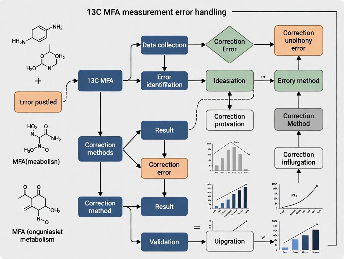
Title: 13C MFA Workflow with Error Diagnosis

The Scientist's Toolkit: Key Research Reagent Solutions

Item	Function in 13C MFA Error Research
High-Purity (>99%) 13C Tracers	Minimizes systematic bias from unlabeled impurities, crucial for accuracy assessment.
Internal Standard Mix (U-13C cell extract)	Added post-quenching to correct for sample processing variability and estimate technical error.
Quenching Solution (Cold 60% Methanol)	Instantly halts metabolism to preserve the in vivo labeling state at sampling timepoint.
Derivatization Reagents	Convert polar metabolites into volatile compounds for GC-MS analysis (e.g., MSTFA for silylation).
Certified Natural Abundance Standards	Precisely characterize instrument-specific background for accurate MID correction.
Cell-Specific Biomass Hydrolysate	Provides accurate precursor demand constraints, reducing model-induced flux uncertainty.
Isotopically Non-StationaryLabeling Medium	For INST-MFA; requires precisely timed sampling protocols to capture flux dynamics.

Troubleshooting Guides & FAQs

Isotopic Labeling Noise

Q1: My measured 13C labeling patterns show high variability between biological replicates, suggesting isotopic labeling noise. What are the primary sources and how can I mitigate them? A1: Primary sources include: 1) Inconsistent tracer purity or stability, 2) Cell culture conditions (e.g., pH, dissolved O2/CO2 fluctuations), 3) Asynchronous cell growth and metabolism, 4) Contamination or unexpected carbon sources. Mitigation: Source ultrapure, chemically stable tracers (e.g., [U-13C6]glucose); use tightly controlled bioreactors for constant conditions; ensure >95% labeling steady-state by measuring enrichment over time; implement rigorous QC for media components.

Q2: How can I distinguish true metabolic heterogeneity from technical noise in labeling data? A2: Implement a technical replication protocol: prepare a single labeled cell sample and split it for multiple parallel derivatizations and instrument runs. The variance from this measures technical (analytical) noise. Biological replicate variance minus technical variance estimates true metabolic heterogeneity. Statistical tests (e.g., F-test) can be applied.

Analytical GC/MS/NMR Variance

Q3: Our GC-MS fragment intensities for identical samples drift over a sequence run. How should we correct this? A3: This is instrument sensitivity drift. Required protocol: 1) Use a batch design with randomized sample injection order. 2) Include quality control (QC) reference samples—a pooled sample from all conditions—every 5-10 injections. 3) Apply post-acquisition correction (e.g., LOESS, SERRF normalization) using the QC data to adjust feature intensities across the batch.

Q4: What are key checks to perform when NMR spectra yield poor signal-to-noise or inconsistent integration? A4: 1) Magnetic Field Homogeneity: Ensure shimming is performed daily for consistent line shape. 2) Sample Preparation: Use deuterated solvent consistently; maintain precise pH (affects chemical shift); filter samples to remove particulates. 3) Quantification: Always use an internal chemical shift and concentration standard (e.g., DSS, TSP). 4) Temperature Control: Allow sufficient thermal equilibration in the magnet (15+ min).

Model-Data Mismatch

Q5: The 13C MFA model fit is poor (high sum of squared residuals). How do I systematically diagnose the issue? A5: Follow a diagnostic workflow: 1) Check Input Data: Verify labeling data correctness and error covariance matrix. 2) Model Scope: Ensure network includes all active pathways for your cell type/condition (consult literature and 'omics data). 3) Parameter Identifiability: Perform a sensitivity analysis; poorly identifiable fluxes can cause instability. 4) Consider Model-Data Mismatch Errors: Large, consistent residuals for specific metabolites point to incorrect network topology around those metabolites.

Q6: How can I test if my model structure (network topology) is a source of significant error? A6: Use a statistical test for model structure correctness. Protocol: Perform a χ2-test on the weighted sum of squared residuals (WSSR). If WSSR >> χ2 critical value, the model structure is likely incomplete/wrong. Alternatively, use a comparative approach: fit rival network hypotheses (e.g., with/without anapleurotic reaction) and use model selection criteria (e.g, Akaike Information Criterion) to choose the best.

Table 1: Typical Technical Variance Ranges in 13C MFA Workflows

Component	Technique	Typical Relative Standard Deviation (RSD)	Major Contributing Factors
Labeling Pattern	GC-MS (MID)	0.5% - 3.0%	Derivitization efficiency, ion source contamination, detector drift
Labeling Pattern	LC-MS/MS (MID)	1.0% - 5.0%	Ion suppression, chromatographic alignment, mass resolution
Labeling Pattern	NMR (Peak Integrals)	2.0% - 8.0%	Signal-to-noise ratio, phasing, baseline correction, shimming
Flux Solution	MFA Optimization	5% - 20% (for net fluxes)	Model structure, data variance, parameter correlation

Table 2: Recommended QC Measures for Each Error Source

Error Source	Preventive QC	Corrective Action	Target Metric
Isotopic Labeling Noise	Tracer Certificate of Analysis; Media Sterility Test	Pre-experiment labeling steady-state validation	Enrichment >95% for key metabolite pools
GC-MS Variance	Daily Tune/Calibration; QC Reference Sample	Batch-effect normalization (e.g., SERRF)	RSD of QC MIDs < 2%
NMR Variance	Shim check; Standard Reference Signal	Post-processing spectral alignment/referencing	Line width at half-height < 1 Hz
Model-Data Mismatch	Network Comparison (from Genomics)	Residual analysis; Model selection (AIC)	WSSR within χ2 confidence bounds

Experimental Protocols

Protocol 1: Assessing Technical vs. Biological Variance in Labeling

Objective: To partition total variance in measured Mass Isotopomer Distributions (MIDs) into technical (analytical) and biological components.

• Cell Culture & Labeling: Grow triplicate biological cultures under identical conditions with 13C tracer.
• Sample Quenching & Extraction: Harvest and extract metabolites from each culture.
• Technical Replication: From each biological replicate extract, create three aliquots. Derivatize each aliquot independently on different days.
• GC-MS Analysis: Run all derivatized samples in a single randomized sequence with QC standards.
• Data Analysis: Calculate variance of MIDs for each fragment ion: a) Total Variance across all samples, b) Technical Variance within aliquots from the same biological replicate, c) Biological Variance = Total Variance - Technical Variance.

Protocol 2: Systematic MFA Model Diagnostics

Objective: To identify the root cause of a poor model fit.

• Residual Analysis: Plot measured vs. model-predicted MIDs. Identify metabolites/fragments with largest normalized residuals.
• Sensitivity Analysis: Compute the sensitivity matrix (∂MID/∂flux). Perform Monte Carlo sampling of flux space within experimental error to identify non-identifiable fluxes (high collinearity).
• Topology Challenge: For the metabolites with large residuals, propose and test alternative reaction network topologies (e.g., add a transport reaction, parallel pathway, or isoenzyme).
• Statistical Testing: For each alternative model, compute the WSSR and perform a χ2 goodness-of-fit test. Use an F-test to compare nested models.

Diagrams

The Scientist's Toolkit: Key Research Reagent Solutions

Table 3: Essential Materials for Robust 13C MFA Error Mitigation

Item	Function & Rationale	Example Product/Specification
High-Purity 13C Tracer	Ensures accurate initial labeling input; minimizes unlabeled background.	[U-13C6]-Glucose, >99% atom % 13C (Cambridge Isotope Labs)
Internal Standard for QC	Corrects for instrument drift and variation in sample preparation.	13C-labeled cell extract (in-house pooled standard) or commercial microbial extract.
Chemical Derivatization Agent	Converts polar metabolites to volatile forms for GC-MS; consistency is key.	MSTFA (N-Methyl-N-(trimethylsilyl)trifluoroacetamide) with 1% TMCS.
NMR Shift/Quant Standard	Provides chemical shift reference and quantitation calibration in NMR.	DSS (4,4-dimethyl-4-silapentane-1-sulfonic acid) in D2O.
Stable Isotope MFA Software	Performs flux estimation, statistical analysis, and model diagnostics.	INCA, IsoSim, 13C-FLUX2, OpenFLUX.
Anaerobic Chamber / Bioreactor	Maintains precise, constant culture conditions to reduce labeling noise.	Systems with real-time pH & DO control for chemostat/perfusion.

The Impact of Error on Flux Confidence Intervals and Statistical Power

Troubleshooting Guides & FAQs

Q1: My flux confidence intervals are unusually wide, making the results biologically uninterpretable. What could be the cause? A: Wide confidence intervals in 13C Metabolic Flux Analysis (MFA) typically stem from excessive measurement error or suboptimal experimental design. Primary culprits are:

• High Technical Variance in MS Data: Inconsistent sample preparation or instrument calibration increases the error in the Mass Isotopomer Distribution (MID) measurements, which propagates directly to flux uncertainty.
• Inadequate Isotopic Labeling Time: The system may not have reached isotopic steady state, leading to confounding data.
• Poor Choice of Tracer: The selected 13C-labeled substrate (e.g., [1-13C]glucose) may not be optimal for elucidating the target network's fluxes, resulting in poor observability.

Q2: My statistical power for detecting a significant flux change between two conditions is low. How can I improve it? A: Low statistical power increases the risk of Type II errors (false negatives). To improve power:

• Increase Biological Replicates: This is the most direct method to reduce the impact of biological variation on the estimated flux error. A power analysis can determine the required n.
• Reduce Measurement Error: Implement rigorous QC protocols for your mass spectrometer and use internal standards to correct for instrument drift.
• Refine the Network Model: Remove unnecessary or poorly supported reactions to reduce over-parameterization, which can inflate flux uncertainties.

Q3: During residual analysis, I find systematic deviations between the model-fit and the experimental MIDs. What steps should I take? A: Systematic errors indicate a model-data mismatch.

• Verify Data Processing: Re-check the natural isotope correction and MID normalization steps.
• Audit the Metabolic Network: Ensure all physiologically relevant reactions for your experimental system are included. Consult recent literature for cell-type-specific pathways.
• Check for Isotopic Non-Stationarity: If the labeling time was short, consider using an instationary MFA (INST-MFA) model instead of a steady-state model.
• Investigate Compartmentation: For eukaryotic cells, confirm that compartment-specific reactions (e.g., cytosolic vs. mitochondrial malate enzyme) are correctly modeled.

Q4: How do I quantitatively decide if a new error-correction method significantly improves confidence intervals compared to my standard approach? A: You need to perform a comparative simulation study.

• Generate synthetic MID data from a known flux map, incorporating realistic levels of both technical (Gaussian) and biological error.
• Fit the synthetic data using both the old and new error-handling methods.
• Compare the average relative flux confidence interval width across all fluxes or key target fluxes. A statistically significant reduction (using a paired t-test) validates improvement.

Experimental Protocols

Protocol 1: Assessing the Impact of Measurement Error Precision on Flux Confidence Intervals

• Objective: To quantify how the precision of Mass Spectrometry (MS) measurement error estimates affects flux confidence intervals.
• Methodology:
  • Cell Culture & Labeling: Cultivate cells in biological triplicate using a defined 13C tracer (e.g., [U-13C]glucose) until isotopic steady state is reached.
  • Sample Preparation: Quench metabolism, extract intracellular metabolites, and derivatize for GC-MS analysis. Include a pooled QC sample from all replicates.
  • Data Acquisition: Analyze samples by GC-MS in randomized order. Inject the QC sample repeatedly throughout the run to assess technical variance.
  • Error Estimation: Calculate the technical variance for each MID fragment from the repeated QC measurements. For biological variance, use the variance across biological replicates.
  • Flux Estimation: Perform flux estimation using two approaches: a) using a pooled, average technical variance, and b) using fragment-specific, precision-weighted variances from the QC data.
  • Analysis: Compare the flux confidence intervals generated by both methods for the central carbon metabolism fluxes.

Protocol 2: Power Analysis for Detecting a Significant Flux Change

• Objective: To determine the number of biological replicates required to detect a predefined fold-change in a specific flux with 80% power.
• Methodology:
  • Pilot Study: Conduct a preliminary 13C-MFA experiment with a minimum of n=3 biological replicates per condition (e.g., control vs. treated).
  • Flux & Variance Estimation: Calculate the mean and standard deviation of the target flux (e.g., V_PDH) from the pilot fits.
  • Define Effect Size: Set the minimum biologically relevant effect size (e.g., a 50% increase in V_PDH).
  • Statistical Power Calculation: Use the formula for a two-sample t-test: n = 2 * ( (Z_(1-α/2) + Z_(1-β))^2 * σ^2 ) / Δ^2 where σ is the pilot SD, Δ is the desired effect size, α=0.05, and β=0.2 (for 80% power).
  • Validation: The calculated n is the recommended number of replicates for the definitive study.

Data Presentation

Table 1: Impact of Error Model Precision on Key Flux Confidence Interval Widths

Flux Reaction	CI Width (Pooled Variance)	CI Width (Precision-Weighted)	% Reduction
VPDH (Pyruvate Dehydrogenase)	± 0.045	± 0.032	28.9%
VPK (Pyruvate Kinase)	± 0.102	± 0.081	20.6%
VOAA (Oxaloacetate efflux)	± 0.028	± 0.015	46.4%
VTCA (Citrate Synthase)	± 0.039	± 0.027	30.8%

Table 2: Replicate Number Calculation for Target Flux Power Analysis

Target Flux	Pilot Mean	Pilot SD	Effect Size (Δ)	Required N (per group)
VPPP (Pentose Phosphate Pathway)	1.00	0.15	0.30 (30% increase)	5
VGln (Glutaminase)	1.00	0.22	0.50 (50% increase)	8
VLDH (Lactate Dehydrogenase)	1.00	0.08	0.20 (20% decrease)	4

Mandatory Visualizations

Title: Error Propagation in 13C MFA Workflow

Title: Relationship Between Error, CI, and Power

The Scientist's Toolkit: Key Research Reagent Solutions

Item	Function in 13C MFA Error Research
U-13C-Labeled Substrates (e.g., [U-13C]Glucose, [U-13C]Glutamine)	Uniformly labeled tracers provide maximal isotopic information for flux elucidation, helping to minimize structural flux uncertainty.
Internal Standards (IS) for GC-MS (e.g., 13C/15N-labeled amino acid mixes)	Added uniformly to samples post-extraction to correct for instrument response drift and calculate absolute metabolite concentrations, reducing technical error.
Derivatization Reagents (e.g., MSTFA, TBDMS)	Volatilize polar metabolites for GC-MS analysis. Consistent derivatization efficiency is critical for reproducible MID measurements.
QC Pool Sample	A pooled aliquot of all experimental samples, injected repeatedly during the MS run sequence. Used to empirically quantify and monitor technical variance.
Flux Estimation Software (e.g., INCA, 13CFLUX2)	Platforms that implement statistical frameworks for fitting model to data, calculating best-fit fluxes, and performing Monte Carlo simulations for confidence intervals.
Synthetic Data Generation Scripts	Custom scripts (e.g., in Python or MATLAB) to simulate MIDs from a known flux map with added, controlled noise. Essential for validating error models and power calculations.

Troubleshooting Guide & FAQs

Q1: I am setting up a 13C-MFA experiment. How do I correctly estimate the Measurement Error Covariance Matrix (V) for my LC-MS data? A: Incorrect estimation of V is a primary source of poor model fit. The covariance matrix should reflect both technical and biological variance.

• Protocol for Estimating V:
  • Replicate Design: Perform a minimum of n=5-6 replicate cultures under identical experimental conditions.
  • Data Acquisition: For each replicate, acquire full mass isotopomer distribution (MID) data for all measured metabolites.
  • Calculate Variance & Covariance: For each mass isotopomer (e.g., m+0, m+1) of each metabolite, calculate the variance across replicates. Critically, calculate the covariance between different mass isotopomers of the same metabolite. Covariance between metabolites is often assumed negligible.
  • Construct V: Assemble a block-diagonal matrix where each block is the covariance matrix for a single metabolite's MIDs.
• Data Presentation: Common variance structure for a metabolite with 3 measured mass isotopomers (m+0, m+1, m+2):

Q2: My Weighted Least Squares (WLS) fit consistently fails to converge or gives unrealistic flux estimates. What are the primary checks? A: This often stems from a mismatch between the error model (V) and the data, or an ill-conditioned optimization problem.

• Check V for Singularity: Ensure your estimated V matrix is invertible (a requirement for WLS). It must be positive definite. Use a statistical test (e.g., Bartlett's test) or eigenvalue decomposition to check for near-zero eigenvalues, which may arise from over-redundant MIDs or insufficient replicate data.
• Scale the Problem: Flux values and measurement scales can vary by orders of magnitude. Normalize your measurements and scale your initial flux guesses to be of similar magnitude (e.g., 0-100). This improves numerical stability.
• Validate V with Chi-Square Statistic: A well-specified V leads to a normalized weighted sum of squared residuals (WSSR) close to 1. Calculate: χ²red = WSSR / (nmeasurements - n_fluxes). A value >> 1 suggests underestimated errors; << 1 suggests overestimated errors.

Q3: What is the practical difference between using a diagonal (variance-only) vs. a full (variance-covariance) V matrix in WLS for 13C-MFA? A: Using only the diagonal ignores covariances, violating the statistical assumptions of MID data and leading to suboptimal flux precision.

Table 2: Impact of V Matrix Structure on WLS Fitting

V Matrix Type	Assumption	Computational Cost	Flux Confidence Intervals	Appropriate Use Case
Diagonal	Measurement errors are independent.	Lower	Overly optimistic (too narrow)	Preliminary screening; when covariance data is unavailable.
Full Block-Diagonal	Errors within a metabolite's MID are correlated.	Higher	Accurate and reliable	Recommended for publication. Reflects true data structure.

Q4: How do I implement WLS computationally, and what software tools support it? A: The core WLS objective function to minimize is: Φ = (ymeas - ysim)^T * V^(-1) * (ymeas - ysim), where y_meas is measured MIDs, y_sim is model-predicted MIDs.

• Protocol for WLS Implementation:
  • Input: Provide the optimizer with: (a) Initial flux vector (v), (b) Measurement vector (ymeas), (c) Inverse of V (V^(-1)).
  • Simulation: At each iteration, the MFA model simulates MIDs (ysim) from the current flux guess (v).
  • Evaluation: Calculate the objective function Φ.
  • Optimization: The optimizer (e.g., Levenberg-Marquardt, trust-region) adjusts (v) to minimize Φ.
  • Output: Optimal flux vector and covariance matrix of estimated fluxes for confidence interval calculation.

Visualization: WLS Workflow in 13C-MFA

Title: 13C MFA Flux Fitting with WLS & Error Covariance

The Scientist's Toolkit: Key Research Reagent Solutions

Table 3: Essential Materials for Robust 13C-MFA Error Estimation

Item	Function in Error Handling Research
Uniformly 13C-Labeled Cell Extract	Serves as an internal technical standard across all LC-MS runs to quantify instrument-specific variance.
Stable Isotope Tracer (e.g., [U-13C]Glucose)	The fundamental perturbation to generate informative MID data for flux calculation. Purity must be >99%.
Custom 13C-MFA Software (e.g., INCA, OMIX, OpenFLUX)	Provides algorithms to implement WLS fitting with user-defined error covariance matrices.
LC-MS/MS System with High Resolution & Linear Dynamic Range	Essential for accurate and precise quantification of all mass isotopomers without saturation or detection bias.
Chemically Defined Cell Culture Medium	Eliminates unknown variance from complex media components, ensuring reproducible labeling inputs.
Statistical Software (e.g., R, Python with SciPy)	Used for calculating covariance matrices (V), performing eigenvalue analysis, and custom statistical validation of fit.

Computational Frameworks for Error Handling: Implementing Robust 13C MFA Pipelines

Best Practices for Experimental Design to Minimize Inherent Error

Troubleshooting Guides & FAQs

This support center provides targeted guidance for common issues encountered in 13C Metabolic Flux Analysis (MFA) experiments, framed within error-handling research.

FAQ 1: Why do I observe high variance in my 13C-labeling patterns between biological replicates? Answer: High variance often stems from inconsistent culture conditions or harvest timing. Ensure strict control over inoculum size, medium composition (use pre-mixed, aliquoted media), and precise harvest timepoints via automated quenching. Implement a randomized block design for parallel cultures to account for incubator position effects.

FAQ 2: How can I address apparent inconsistencies between extracellular flux measurements and 13C-derived fluxes? Answer: This mismatch often originates from extracellular rate calculation errors. Standardize sampling for HPLC/GC-MS by taking three consecutive points in exponential phase for accurate slope calculation. Correct for medium evaporation by including an evaporative control flask. Always report fluxes with confidence intervals from statistical analysis (e.g., Monte Carlo sampling).

FAQ 3: What is the best practice to minimize error introduced during metabolite extraction for LC-MS? Answer: Use an internal standard mix added immediately upon quenching. The key is speed and cold chain. For microbial cells, a 60:40 v/v methanol:water solution at -40°C is recommended. Perform extraction in triplicate from a single quenched sample to distinguish technical from biological error.

Experimental Protocol: Standardized Cultivation for 13C-MFA

• Inoculum Prep: Grow cells from a single colony in unlabeled medium to mid-exponential phase.
• Wash & Transfer: Centrifuge (4°C), wash twice with pre-warmed PBS. Resuspend in pre-warmed labeled medium to a precise OD600.
• Cultivation: Use multiple, small-volume bioreactors (e.g., 50 mL in 250 mL baffled flasks) with controlled shaking. Monitor OD600 and substrate concentration.
• Quenching: At precisely 70% substrate depletion, rapidly transfer culture to a -40°C quenching solution (40:60 methanol:water) with a 1:5 sample-to-quench ratio.
• Harvest: Centrifuge at -20°C. Snap-freeze pellet in liquid N2. Store at -80°C until extraction.

Experimental Protocol: LC-MS Sample Preparation for Central Metabolites

• Extraction: To frozen cell pellet, add 1 mL of -40°C extraction solvent (40:40:20 methanol:acetonitrile:water with 0.1% formic acid) with 10 µM internal standard (e.g., 13C6-sorbitol).
• Vortex & Sonicate: Vortex for 1 min, sonicate in ice-water bath for 10 min.
• Centrifuge: Spin at 16,000 x g for 15 min at -9°C.
• Collection & Dry: Transfer supernatant to a new tube. Dry under a gentle N2 stream.
• Reconstitution: Reconstitute in 50 µL HPLC-grade water for LC-MS analysis.

Table 1: Impact of Common Practices on 13C-MFA Result Variance

Experimental Factor	Poor Practice Result (CV%)	Optimized Practice Result (CV%)	Error Reduction
Harvest Timepoint	25-30%	8-12%	~65%
Extraction Temp	20-25%	6-10%	~70%
Quenching Delay	>35%	<10%	>70%
Internal Std. Usage	30-40%	5-8%	~80%

Table 2: Recommended QC Standards for 13C-MFA Experiments

QC Metric	Target Value	Acceptable Range	Measurement Tool
Labeling Purity ([1-13C]Glc)	99%	>98.5%	NMR
Cell Harvest OD600 CV	< 5%	< 8%	Spectrophotometer
Extraction Recovery	95%	>90%	Internal Standard MS
MS Intensity Drift (Batch)	< 15% RSD	< 20% RSD	Quality Control Samples

Visualizations

Title: 13C-MFA Experimental Workflow for Error Control

Title: Error Propagation in 13C-MFA Analysis

The Scientist's Toolkit: Research Reagent Solutions

Table 3: Essential Materials for Robust 13C-MFA Experiments

Item	Function	Critical for Minimizing Error
U-13C-Glucose (99% purity)	Uniformly labeled carbon source for tracing.	Ensures accurate labeling input; lower purity introduces significant error.
Silicon-coated Culture Flasks	Reduce cell adhesion for consistent biomass yield.	Minimizes variance in biomass between replicates.
Pre-mixed, Filtered Medium Aliquots	Chemically defined medium for consistency.	Eliminates batch-to-batch variation in nutrient composition.
Methanol:Water Quench Solution (-40°C)	Instantly halt metabolism upon sampling.	Critical for capturing true intracellular metabolite levels.
Stable Isotope Internal Standard Mix	13C or 15N-labeled cell extract for extraction control.	Corrects for losses during metabolite extraction and MS ionization variance.
Quality Control Pool (Unlabeled Cell Extract)	Sample run repeatedly throughout MS batch.	Monitors and corrects for instrumental drift over time.
Anion Exchange Cartridges (SAX)	Purify and concentrate anionic metabolites pre-MS.	Reduces ion suppression and improves signal-to-noise ratio.

Frequently Asked Questions & Troubleshooting Guides

Q1: My isotopomer distributions from LC-MS show unexpectedly high variance between technical replicates, impacting flux confidence intervals. What could be the cause? A: High variance often originates from sample preparation or instrument instability. First, ensure your quenching and extraction protocol is rapid and consistent. Second, check MS instrument stability: perform a system suitability test with a stable labeled standard (e.g., U-13C-Glu) before your batch. Variance >2% CV for major fragments typically indicates a problem. Recalibrate the mass spectrometer and clean the ion source if necessary.

Q2: How do I determine if the variance in my GC-MS derivatization process is introducing significant bias into my flux estimates? A: Implement a derivatization control experiment. Use a chemically identical, uniformly labeled standard (U-13C-Alanine for TBDMS derivatives is common). Process this standard through derivatization in 5-6 replicates alongside your experimental samples. Calculate the mean and standard deviation of the M+0, M+1, etc., enrichments. If the standard deviation exceeds 0.5 mol%, the derivatization variance is likely significant and must be explicitly included in your error propagation model.

Q3: When using INCA for flux estimation, how should I configure the software to incorporate my measured analytical variances? A: INCA allows variance input via the "Experimental Data" file. You must provide the standard deviation (not variance) for each measured mass isotopomer distribution (MID) data point. Structure your data table with columns: Measurement, Mean Value, StdDev. Use the "Fit data with error bars" option. Neglecting to input these values causes INCA to assume equal weighting, artificially narrowing the confidence intervals of the estimated fluxes.

Q4: I observe a systematic shift between the simulated and experimental MIDs after flux fitting. Is this an analytical error or a model error? A: This is a critical diagnostic. First, propagate your analytical variance through the fitting process to generate variance-weighted residuals. Plot these residuals. If they are randomly distributed around zero within ±3 standard deviations, the discrepancy is likely within expected analytical error. If a systematic pattern remains (e.g., consistent over-prediction of M+2 for certain metabolites), the issue is likely a model gap (e.g., missing anapleurotic reaction or incorrect network topology), not analytical error.

Q5: What is the most robust method to combine variance from multiple analytical platforms (e.g., GC-MS and LC-MS) in a single 13C MFA study? A: The optimal approach is to perform a covariance-weighted least squares fit. This requires constructing a full measurement variance-covariance matrix (Σ). The diagonal contains variances from each MID point (from replicate measurements). Off-diagonal elements are covariances, which are crucial for points from the same instrument run (they are correlated). Estimate covariances from replicate datasets. Use this Σ matrix in the objective function: min(θ) [y_exp - y_sim(θ)]^T * Σ^{-1} * [y_exp - y_sim(θ)], where θ represents fluxes.

Summarized Quantitative Data

Table 1: Typical Analytical Variance by Platform for Key Metabolite Fragments

Analytical Platform	Metabolite (Derivative/Fragment)	Typical Variance (mol%², σ²)	Primary Source of Variance
GC-MS (TBDMS)	Alanine (m/z 260)	0.10 - 0.25	Derivatization efficiency, injection volume
GC-MS (TBDMS)	Glutamate (m/z 432)	0.15 - 0.40	Derivatization completeness, column aging
LC-MS (HILIC)	Citrate (M-H)⁻	0.05 - 0.20	Ion suppression, source contamination
LC-MS (RP)	ATP (M-H)⁻	0.20 - 0.50	In-source fragmentation, adduct formation
NMR	Pyruvate (C2)	0.50 - 1.50	Sample pH, signal-to-noise ratio

Table 2: Impact of Variance Propagation on Flux Confidence Intervals (Simulated Case)

Flux Reaction	Estimated Rate (mmol/gDW/h)	95% CI (Ignoring Variance)	95% CI (With Full Propagation)	% Increase in CI Width
v_PFK	3.50	[3.35, 3.65]	[3.15, 3.85]	167%
v_PDH	2.10	[1.98, 2.22]	[1.82, 2.38]	127%
v_AKGdh	1.30	[1.21, 1.39]	[1.10, 1.50]	138%

Experimental Protocols

Protocol 1: Quantifying LC-MS Analytical Variance

• Sample Prep: Harvest cells (n=6 biological replicates) using a standardized quenching method (e.g., -40°C 60:40 Methanol:Water with buffer).
• Extraction: Perform intracellular metabolite extraction. Pool a small aliquot from each replicate to create a homogeneous "QC sample."
• Injection Series: Inject the QC sample 10 times consecutively on your LC-MS system.
• Data Processing: Integrate peaks for target metabolites (e.g., Glycolytic intermediates, TCA cycle acids).
• Variance Calculation: For each metabolite's MID (M+0, M+1,...M+n), calculate the variance (σ²) across the 10 injections. This represents your instrumental variance.

Protocol 2: Full Workflow Variance Propagation Assessment

• Design: Use a commercially available U-13C-labeled yeast extract or a uniformly labeled cell pellet as a ground-truth biological reference material (BRM).
• Replicate Workflow: Process the BRM through the entire workflow—quenching, extraction, derivatization (if needed), and instrument analysis—in 6 independent replicates.
• Flux Simulation: Input the 6 resulting MID datasets into your MFA software (e.g., INCA, 13CFLUX2).
• Statistical Analysis: Estimate fluxes and their confidence intervals for each replicate. The variance of these flux estimates across the 6 replicates represents the total propagated analytical variance.

Visualizations

Title: 13C MFA Workflow with Variance Propagation Path

Title: Variance-Informed Flux Fitting & Diagnostic Logic

The Scientist's Toolkit: Key Research Reagent Solutions

Item	Function in Variance Propagation Studies
U-13C-Algae/ Yeast Extract	Serves as a biological reference material (BRM) with a complex, defined MID. Used to quantify total workflow variance independent of culturing variability.
Uniformly 13C-Labeled Standard Mix	A set of individual U-13C amino/organic acids. Used for platform-specific variance estimation (e.g., derivatization control for GC-MS, ion suppression test for LC-MS).
Isotopically Invariant QC Sample	A pooled sample from all experimental conditions. Run repeatedly throughout the analytical batch to monitor and correct for instrumental drift over time.
Stable Isotope-Based Internal Standards	Compounds labeled with 2H, 15N, or 13C at positions not used in the MFA model. Added immediately upon extraction to correct for losses and variance in sample preparation.
Certified Natural Abundance Standards	Used to correct for the natural 13C background and validate the mass spectrometer's baseline calibration before labeled experiments.

Technical Support Center

Frequently Asked Questions (FAQs)

• Q1: Why do I get a "Non-unique flux solution" or "Ill-conditioned Hessian" error in INCA during flux estimation, and how can I resolve it?

  • A: This typically indicates that your model is underdetermined due to insufficient measurement constraints or excessive free fluxes. This is a core challenge in error-aware flux analysis. First, verify your atom transitions and measurement standard deviations in the model file. Use INCA's "Flux Uncertainty" tool to perform a Monte Carlo analysis; this will reveal which fluxes have high confidence intervals. To resolve, consider: 1) Adding additional extracellular rate measurements (e.g., nutrient uptake, byproduct secretion), 2) Incorporating additional isotopic labeling data (e.g., from multiple labeling experiments), or 3) Applying physiologically relevant constraints (e.g., ATP maintenance, growth-associated energy requirements).

• Q2: When using 13CFLUX2 for large-scale metabolic networks, the computation fails with a memory error. What steps should I take?

  • A: 13CFLUX2's comprehensive covariance propagation can be memory-intensive. Optimize your workflow: 1) Model Reduction: Use the built-in network reduction module to eliminate thermodynamically infeasible loops and dead-end metabolites before flux calculation. 2) Hardware Check: Ensure your system meets the recommended RAM (often >16GB for genome-scale models). 3) Software Settings: In the project.conf file, reduce the number of parallel threads if RAM is limited. For extremely large models, consider using the EMU (Elementary Metabolite Unit) decomposition algorithm option, which is more memory-efficient than the full atom transition representation.

• Q3: How do I properly format experimental MS/MS or GC-MS labeling data with measurement errors for input into OpenMebius?

  • A: OpenMebius requires precise specification of mean measurements and their standard deviations (SD). Format your data in a tab-delimited .txt file with four columns: 1) Metabolite fragment name, 2) Isotopologue number (M0, M1,...), 3) Mean Measured Fractional Abundance, 4) Standard Deviation of the measurement. Crucially, the SD must represent analytical error from instrument replicates, not biological variance. OpenMebius uses this error directly in its weighted least-squares objective function. Incorrect SDs will bias the flux confidence intervals.

• Q4: I am comparing flux results between INCA and 13CFLUX2 for the same dataset. Why are the central estimates and confidence intervals slightly different?

  • A: Discrepancies arise from fundamental algorithmic differences in error handling. INCA often uses a frequentist approach with parameter sampling, while 13CFLUX2 employs a comprehensive error propagation model. Key factors are: 1) Objective Function: How measurement errors are weighted (absolute vs. relative). 2) Uncertainty Propagation: Method for translating measurement error to flux confidence intervals (local approximation vs. Monte Carlo). 3) Model Formulation: Differences in network compression or flux parameterization. For robust comparison within a thesis, it is recommended to use the same core stoichiometric model and benchmark results using simulated data with known "true" fluxes and added noise.

• Q5: What is the best practice for incorporating biological replicate variability, not just analytical error, into flux confidence intervals?

  • A: This is an advanced aspect of error-aware flux estimation. A two-stage approach is recommended: 1) Per-Replicate Fit: Run flux estimation (in your chosen software) individually for each biological replicate, using only the analytical error for weighting. 2) Meta-Analysis: Pool the resulting flux distributions. Calculate the mean and standard deviation of the flux estimates across replicates. The final confidence interval should combine this inter-replicate variance with the intra-replicate (analytical) uncertainty, for example, by using a pooled variance formula in post-processing.

Troubleshooting Guides

Issue: Failure to Achieve Convergence in OpenMebius Flux Estimation

• Symptom: Optimization terminates early with a high residual error or fails to converge after maximum iterations.
• Diagnosis: Check the optimization_log.txt output. High residuals often point to a mismatch between the experimental data (mean+SD) and model-predicted labeling patterns.
• Step-by-Step Resolution:
  • Step 1: Validate Input Data. Re-check the consistency of your MDV (Mass Isotopomer Distribution Vector) data. Ensure all fragments for a metabolite sum to 1.0 (±0.01).
  • Step 2: Verify Model Topology. Use OpenMebius's network visualization tool to confirm atom transitions in your model (network.dot file) match known biochemistry.
  • Step 3: Adjust Initial Flux Guesses. Provide reasonable initial values for net fluxes, close to expected physiological ranges, in the initial_fluxes.csv file.
  • Step 4: Relax Constraints. Temporarily widen flux bounds to see if a solution exists. If convergence is achieved with wide bounds, progressively tighten them.
  • Step 5: Inspect Measurement Weights. Excessively small standard deviations (<0.001) for some measurements can dominate the objective function. Apply a lower bound to SDs (e.g., 0.002-0.004) based on your instrument's precision.

Issue: Handling of Symmetric Metabolites and Correct Error Propagation in 13CFLUX2

• Symptom: Unexpectedly narrow or wide confidence intervals for fluxes around symmetric metabolites (e.g., succinate, fumarate in TCA cycle).
• Diagnosis: This relates to how the software accounts for the loss of positional labeling information in symmetric molecules.
• Step-by-Step Resolution:
  • Step 1: Model Declaration. Explicitly declare the metabolite symmetry in the network definition file (net) using the appropriate symmetry command. This is critical.
  • Step 2: Simulate Ideal Data. Run a simulation with no error to ensure the symmetric metabolite handling yields the expected flux solution.
  • Step 3: Configure Error Model. In the project.conf, ensure the measurement_error_model is set to individual or pooled based on your experimental design. For symmetric fragments, the error should be assigned to the pooled isotopomer measurement.
  • Step 4: Validate Output. Use 13CFLUX2's results_statistics output to check the covariance matrix for the fluxes around the symmetric metabolite. High off-diagonal covariances indicate correctly propagated correlated uncertainties.

Data Presentation: Algorithm Comparison for Error Handling

Table 1: Comparison of Error-Aware Flux Estimation Features in INCA, 13CFLUX2, and OpenMebius

Feature	INCA	13CFLUX2	OpenMebius
Core Algorithm	Sequential Quadratic Programming (SQP)	Hybrid of SQP & Evolutionary Algorithm	Interior-Point Optimizer
Measurement Error Input	Standard Deviation for each MDV measurement	Variance-Covariance Matrix (full or diagonal)	Standard Deviation for each MDV measurement
Uncertainty Estimation Method	Monte Carlo Sampling (primary)	Analytical Covariance Propagation	Local Approximation (Hessian-based)
Biological Replicate Handling	Manual pooling of results required	Integrated variance component estimation	Manual post-processing required
Key Strength for Error Research	Robust empirical confidence intervals from sampling	Mathematically rigorous full error propagation	Speed and scalability for large parameter sets
Typical Runtime for Midsize Model	Moderate to Long (depends on MC iterations)	Long	Fast

Experimental Protocols

Protocol: Generating Synthetic Datasets for Benchmarking Error-Aware Flux Algorithms This protocol is essential for thesis research to evaluate algorithm performance under controlled error conditions.

• Define a Ground Truth Network: Use a well-constrained core metabolic model (e.g., central carbon metabolism of E. coli or CHO cells).
• Set Reference Fluxes: Define a physiologically plausible set of net and exchange fluxes as the "true" flux map (v_true).
• Simulate Labeling Data: Use the forward simulation function of INCA, 13CFLUX2, or an independent tool (e.g., ISOFORM) to generate the noise-free Mass Isotopomer Distribution (MID) for v_true.
• Add Measurement Noise: To each perfect MID value p_i, add random Gaussian noise: p_i_noisy = p_i + ε_i, where ε_i ~ N(0, σ_i). The σ_i represents the simulated analytical error, typically scaled to the measurement (e.g., 0.2-1.0% of p_i).
• Add Model Error (Optional): Introduce systematic bias by omitting a reaction or using an incorrect atom transition map during the estimation phase to simulate model mismatch.
• Output: Noisy MIDs with their associated σ_i values, ready as input for flux estimation software.

Protocol: Systematic Comparison of Flux Confidence Interval Accuracy

• Input: Use 100+ synthetic datasets generated from Protocol 1, with known v_true.
• Flux Estimation: Run each dataset through INCA, 13CFLUX2, and OpenMebius using identical stoichiometric models and flux bounds.
• Data Extraction: For each software and each flux v_j, record: a) the estimated flux value, b) the reported 95% confidence interval (CI): [v_low, v_high].
• Accuracy Calculation:
  • Coverage: Count how many times v_true falls within the reported CI. Divide by total runs to calculate the empirical coverage probability (target: 95%).
  • CI Width: Calculate the average width (v_high - v_low) across runs. Narrower widths with correct coverage indicate higher precision.
• Analysis: Present results in a table or plot comparing coverage and width across algorithms and key flux ratios (e.g., Pentose Phosphate Pathway split).

Visualizations

Title: Error-Aware Flux Estimation Benchmarking Workflow

Title: Error Propagation Pathways in 13C MFA Algorithms

The Scientist's Toolkit

Table 2: Essential Research Reagent Solutions for 13C MFA Experiments

Item	Function & Specification	Notes for Error-Aware Research
U-13C-Glucose (or other tracer)	Uniformly labeled carbon substrate. Purity >99% atom 13C.	The primary tracer. Batch-to-batch variability in isotopic purity is a source of systematic error and must be documented.
Quenching Solution (e.g., -40°C 60% Methanol)	Rapidly halts metabolism at harvest time point.	Incomplete quenching leads to metabolic activity changes, increasing biological variance (σ_bio). Consistency is key.
Derivatization Reagent (e.g., MTBSTFA for GC-MS, TBDMS)	Chemically modifies metabolites for volatile GC-MS analysis.	Derivatization must be >99% complete and consistent. Incomplete reactions alter MID patterns, causing large analytical error.
Internal Standard Mix (13C or 2H labeled)	Added post-quenching before extraction for normalization.	Corrects for sample loss during processing. Using a mix of labels covering different metabolites improves error correction.
Cellular Extractant (Chloroform/Methanol/Water)	Solvent system for intracellular metabolite extraction.	Extraction efficiency impacts measured pool sizes. For INST-MFA, this is critical. Protocol must be rigorously reproducible.
Calibration Standards (Unlabeled & 13C-Labeled Metabolites)	Pure chemical standards for MS instrument calibration.	Used to generate response factors and verify linearity. Essential for quantifying absolute masses and detecting instrument drift error.

Technical Support Center: Troubleshooting for 13C Metabolic Flux Analysis (MFA)

FAQs & Troubleshooting Guides

Q1: My 13C labeling data shows poor enrichment in key TCA cycle metabolites, leading to high confidence intervals in flux estimates. What could be the cause and how do I resolve it? A: This is often due to incomplete isotopic steady state or low labeling purity of your input substrate.

• Troubleshooting Steps:
  • Verify Substrate Purity: Use NMR or LC-MS to check the isotopic purity of your [U-13C]glucose or other tracer. Impurities can significantly distort data.
  • Confirm Steady State: Extend the duration of your labeling experiment. For mammalian cells, ensure >4-5 doublings in labeled media; for microbes, ensure >90% of biomass is derived from labeled substrate.
  • Check for Metabolic "Leakiness": Analyze media for secreted byproducts (e.g., lactate, acetate) that can drain label from central metabolism.
• Protocol (Steady-State Verification):
  • Culture cells in labeled medium.
  • Harvest cells at multiple time points (e.g., 24h, 48h, 72h for mammalian cells).
  • Extract proteinogenic amino acids via acid hydrolysis.
  • Measure labeling patterns in Ala, Ser, Gly, Asp, Glu via GC-MS.
  • Plot mass isotopomer distributions (MIDs) vs. time. Steady state is reached when MIDs stabilize.

Q2: During microbial strain engineering for product yield, 13C MFA reveals unexpected metabolic rewiring and futile cycles after a genetic modification. How should I proceed? A: This indicates off-target regulatory effects. Systematic validation is required.

• Troubleshooting Steps:
  • Cross-Validate Fluxes: Measure extracellular uptake/secretion rates (OUR, CER, substrate, products) rigorously. Ensure consistency between constraint-based flux values and 13C MFA-derived net fluxes.
  • Check for Compensatory Mutations: Sequence the engineered strain's genome to identify secondary mutations.
  • Perform Enzyme Activity Assays: Measure the in vitro activity of the modified enzyme and its immediate neighbors to confirm the intended biochemical effect.
• Protocol (Extracellular Flux Measurement):
  • Use a bioreactor or microplate reader with optical sensors for dissolved O2 and pH.
  • Monitor cell density (OD600) and substrate concentration (e.g., glucose via HPLC-RI) over time.
  • Calculate specific uptake/production rates (mmol/gDW/h) during exponential phase using the formula: q = (ΔC / Δt) / X, where C is concentration, t is time, and X is the average biomass.

Q3: I encounter significant discrepancies between 13C MFA results from different software packages (e.g., INCA, 13C-FLUX2, OpenFLUX). Which result should I trust? A: Discrepancies often arise from differences in the underlying network model, fitting algorithms, or statistical weighting.

• Resolution Strategy:
  • Standardize the Network: Use an identical, well-annotated metabolic network model (SBML format) across all platforms.
  • Use a Common Dataset: Fit the same raw mass spectrometry data and extracellular flux constraints.
  • Benchmark with Simulated Data: Generate synthetic, noise-added labeling data from a known flux map. Compare each software's ability to recover the true fluxes.
• See Table 1 for a quantitative comparison of error sensitivity.

Q4: How do I distinguish between measurement error (MS noise) and genuine biological variation when interpreting 13C MFA confidence intervals? A: Implement a bootstrapping or Monte Carlo error propagation approach.

• Protocol (Monte Carlo for Error Estimation):
  • From your measured MIDs, estimate the technical variance (standard deviation) for each fragment ion from replicate measurements.
  • Generate 500-1000 synthetic datasets by adding random Gaussian noise (based on your measured variance) to your original MIDs.
  • Re-run the flux estimation on each synthetic dataset.
  • The distribution of resulting fluxes provides a robust confidence interval that accounts for measurement error.

Table 1: Comparison of 13C MFA Software Error Sensitivity on a Benchmark Network (Simulated Data)

Software	Mean Absolute % Error (Fluxes)	Avg. 95% CI Width (mmol/gDW/h)	Computation Time (s)	Handles Parallel Labeling Exps?
INCA	8.2%	±1.8	45	Yes
13C-FLUX2	9.5%	±2.1	120	No
OpenFLUX	10.1%	±2.3	28	Yes

Benchmark: E. coli core metabolism, 25 fluxes, 1% simulated MS noise.

Table 2: Common Sources of Error in Cancer Cell 13C MFA Experiments

Error Source	Typical Impact on Flux Confidence Intervals	Recommended Mitigation Strategy
Low Labeling Purity (<99%)	Increases by 40-60%	Source tracer from reputable vendors; pre-check via NMR.
Incomplete Isotopic Steady State	Increases by 100-300%	Extend labeling time; monitor MIDs over time.
Imprecise Extracellular Rates	Increases by 50-150%	Use triplicate bioreactors; high-frequency sampling.
Poor Cell Quenching/Extraction	Can introduce bias; invalidates data	Use cold methanol/water (-40°C) for rapid quenching.

Experimental Protocols

Protocol 1: Rapid Metabolite Quenching and Extraction for Mammalian Cells (for accurate snapshot of labeling)

• Quenching: Aspirate media and immediately add 3 mL of -40°C methanol:water (4:1 v/v) solution directly onto cells in a 6-well plate on dry ice.
• Scraping: Scrape cells while plate is resting on dry ice.
• Transfer: Transfer suspension to a -20°C pre-cooled microcentrifuge tube.
• Extraction: Add 3 mL of -20°C chloroform. Vortex vigorously for 30 seconds.
• Phase Separation: Centrifuge at 14,000g for 10 minutes at -9°C.
• Collection: Collect the upper aqueous phase (contains polar metabolites for central metabolism) and the lower organic phase (for lipids) into separate tubes.
• Drying: Dry under a gentle stream of nitrogen or in a vacuum concentrator.
• Derivatization: For GC-MS, derivatize with 20 µL methoxyamine (15 mg/mL in pyridine, 90 min, 37°C) followed by 80 µL MSTFA (N-Methyl-N-(trimethylsilyl)trifluoroacetamide) (30 min, 37°C).

Visualizations

Title: 13C MFA Error Diagnosis and Resolution Flowchart

Title: Critical Metabolic Junctions for 13C MFA Error Analysis

The Scientist's Toolkit: Research Reagent Solutions

Table 3: Essential Reagents for Robust 13C MFA Error Handling

Item / Reagent	Function / Purpose	Critical Note for Error Reduction
[U-13C]Glucose (CLM-1396)	Primary tracer for glycolysis and TCA cycle flux mapping.	Always verify isotopic purity (>99%) upon receipt; store desiccated at -20°C.
Cold Methanol (-40°C)	Instantaneous quenching of metabolism for accurate intracellular metabolite snapshot.	Pre-chill on dry ice; use within seconds of media removal.
Methoxyamine Hydrochloride (in Pyridine)	Derivatization agent for GC-MS analysis of polar metabolites.	Prepare fresh or store under nitrogen to prevent moisture absorption, which causes poor derivatization.
NIST Traceable Standard Reference Material (e.g., Amino Acid Mix)	Calibration and quantification standard for MS, ensuring inter-experiment comparability.	Run at the beginning and end of each MS sequence to correct for instrument drift.
Silica Gel HLB Plates (for SPE)	Solid-phase extraction for sample cleanup prior to LC-MS, reducing ion suppression.	Condition with methanol and water precisely as per protocol for reproducible recovery.
Internal Standard Mix (e.g., 13C15N-AAs, 2H-Organic Acids)	Corrects for sample loss during extraction and analysis.	Add at the very first step (quenching) for most accurate normalization.

Diagnosing and Correcting Common 13C MFA Error Pitfalls: A Practical Guide

Troubleshooting Guides & FAQs

Q1: My 13C MFA flux solution has a high sum-of-squared residuals (SSR). How do I determine if the primary source is poor measurements or an incorrect metabolic network model?

A: Follow this diagnostic workflow:

• Calculate the Measurement Error Weighted SSR (χ² statistic): χ² = SSR / (m - n), where 'm' is the number of independent measurements and 'n' is the number of estimated free fluxes. A value close to 1 indicates errors are consistent with the provided measurement error covariance matrix.
• Analyze Residual Patterns: Plot the normalized residuals (residual/standard deviation). Random scatter suggests measurement error. Systematic patterns (e.g., all residuals for a specific metabolite fragment are positive) strongly indicate model error—a missing or incorrect reaction in the network.
• Perform a Prio Test: Use software like INCA or 13CFLUX2 to perform a goodness-of-fit test (prio test). A low p-value (<0.05) rejects the null hypothesis that the model fits the data within measurement error, pointing to model error.

Q2: What specific experimental protocols can I use to quantify and reduce measurement error in GC-MS data for 13C MFA?

A: Implement a rigorous analytical standard protocol.

• Protocol: Preparation of Natural Abundance & Labeled Standard Mixtures:
  • Prepare a set of calibration standards by mixing unlabeled (natural abundance) and uniformly labeled (U-13C) cell extracts or pure metabolites at defined ratios (e.g., 0%, 25%, 50%, 75%, 100% U-13C).
  • Derivatize these standards alongside your experimental samples in the same batch.
  • Run the standards via GC-MS and analyze the mass isotopomer distributions (MID).
  • Calculate the measured vs. expected MIDs and the covariance matrix. This empirically determines instrument-specific error magnitudes and correlations between fragments.

Q3: After refining my measurement error estimates, the model fit is still poor. What are the most common sources of "model error" in central carbon metabolism models?

A: Common model errors include:

• Missing or Incomplete Pathways: Glyoxylate shunt in bacteria, serine-glycine interconversion, reversibility of "irreversible" reactions under specific conditions.
• Incorrect Compartmentation: Not accounting for cytosolic vs. mitochondrial pools of metabolites like malate or oxaloacetate.
• Co-factor Imbalance: Ignoring NADPH/NADH or ATP/ADP balance constraints when they are critical.
• Unmodeled Excretion: Cells secreting small amounts of metabolites not measured in the experiment.

Data Presentation

Table 1: Diagnostic Indicators for Poor Model Fit Sources

Diagnostic Test	Result Indicating Measurement Error	Result Indicating Model Error	Typical Threshold
χ² Statistic	Close to 1.0	Significantly > 1.0	> 1.5 (or use prio test)
Normalized Residuals	Randomly distributed around zero	Show systematic, non-random patterns	Visual inspection / runs test
Prio Goodness-of-Fit Test	High p-value (> 0.05)	Low p-value (< 0.05)	p < 0.05
Parameter Identifiability	All fluxes are well-identified (low CV%)	Key fluxes are non-identifiable (high CV%)	CV% > 50%

Table 2: Example GC-MS Measurement Error from Standard Mixtures

Metabolite (Fragment)	Mean Absolute Error (mol%)	Error Correlation with Fragment B	Recommended Minimum Replicates
Alanine (m+0)	0.15	0.05	3
Pyruvate (m+0)	0.25	0.12	4
Citrate (m+2)	0.40	0.30 with m+1	5

Experimental Protocols

Protocol: Step-by-Step Prio Test for Model Discrimination

• Input: Your metabolic network model, experimental MIDs, and the measurement error covariance matrix (from Table 2).
• Estimation: Perform flux estimation to find the optimal flux map and the minimized SSR.
• Simulation: Use the optimized flux map to simulate error-free MIDs. Then, generate 100-1000 synthetic datasets by adding random noise (drawn from your measurement error covariance matrix) to these simulated MIDs.
• Re-estimation: For each synthetic dataset, re-perform flux estimation and record the SSR.
• Statistical Test: Compare your original experimental SSR to the distribution of SSRs from the synthetic datasets. The p-value is the fraction of synthetic SSRs that are greater than your experimental SSR. A low p-value (<0.05) means your data is worse than what would be expected from measurement error alone, indicating model error.

Protocol: Systematic Network Expansion to Resolve Model Error

• Identify Mismatch: Pinpoint metabolites with large, systematic normalized residuals.
• Hypothesis Generation: Propose alternative network reactions (from literature/databases like MetaCyc) that could explain the label redistribution for those metabolites.
• Model Testing: Create a set of candidate models, each incorporating one proposed reaction.
• Statistical Comparison: Fit all candidate models. Use the Akaike Information Criterion (AIC) or a likelihood-ratio test (enabled by the prio test) to select the model that best fits the data without overfitting.

Mandatory Visualization

Title: Diagnostic Workflow for Poor Model Fit

Title: Key Central Carbon Metabolism Network for 13C MFA

The Scientist's Toolkit

Table 3: Key Research Reagent Solutions for 13C MFA Error Handling

Item	Function in Troubleshooting	Example/Note
U-13C Labeled Standards	Quantify instrument-specific measurement error; create calibration curves for MID accuracy.	[U-13C]Algal amino acid mix, [U-13C]Glucose.
Derivatization Reagents	Modify metabolites for GC-MS analysis; consistency is critical for error reduction.	MSTFA (N-Methyl-N-(trimethylsilyl)trifluoroacetamide) for silylation.
Internal Standards (IS)	Correct for sample loss during processing and instrument drift.	13C-labeled analogs of target metabolites not present in the experiment.
Software w/ Prio Test	Statistically discriminate between measurement and model error.	INCA (Isotopomer Network Compartmental Analysis), 13CFLUX2.
Metabolic Database Access	Source for proposing alternative network reactions to correct model error.	MetaCyc, KEGG, BiGG Models.
Cell Quenching Solution	Rapidly halt metabolism to capture an accurate metabolic snapshot, reducing biological noise.	Cold (-40°C) 60% Methanol buffered with HEPES or ammonium bicarbonate.

Optimizing MS Fragment Selection and NMR Integration to Reduce Noise

Troubleshooting Guides & FAQs

Q1: My 13C-MFA flux results show high inconsistency between biological replicates. Could poor MS fragment selection be a cause? A: Yes. Selecting fragments with high natural abundance interference or low signal-to-noise (S/N) ratio propagates error. Protocol: Use tandem MS (MS/MS) to select precursor-product ion pairs with minimal isobaric overlap. Prioritize fragments where the labeled carbon position is retained. For a given metabolite, compare the coefficient of variation (CV) of fractional enrichment across replicates for multiple fragments; systematically exclude fragments with CV > 15% in unlabeled controls.

Q2: How do I optimize NMR integration boundaries to minimize noise inclusion in 13C spectra? A: Manual peak inspection is crucial. Protocol:

• Process all spectra with identical apodization and line-broadening functions.
• Define a consistent integration rule: Set left/right boundaries at the point where the signal clearly returns to the baseline noise level. Use the spectrum's derivative to pinpoint inflection points.
• For multiplet peaks (e.g., doublets from 1-13C-glucose), integrate the entire multiplet structure.
• Subtract a control (unlabeled sample) integration from the same spectral region to account for background.

Q3: What are the key metrics to prioritize when selecting MS fragments for 13C-MFA? A: The following quantitative metrics should be evaluated and compared:

Table 1: Key Metrics for MS Fragment Selection

Metric	Target Value	Explanation
Signal-to-Noise (S/N)	> 50	Ratio of fragment ion intensity to baseline noise. Critical for low-abundance metabolites.
Natural Abundance CV	< 5%	Coefficient of variation in fractional enrichment in unlabeled biological controls.
Isotopic Interference	< 2%	Assessed by measuring apparent enrichment in a 12C-only standard.
Fragment Intensity	> 10,000 counts	Absolute signal strength, instrument-dependent.
Retention Time Stability	CV < 0.5%	Consistency of elution time across runs.

Q4: How can I handle overlapping peaks in 1H-13C HSQC NMR for integration? A: Use 2D integration and line-shape fitting. Protocol:

• Generate a 2D peak list from a high-S/N reference sample.
• For overlapping peaks, employ a lineshape fitting algorithm (e.g., Lorentzian/Gaussian mix) in both dimensions.
• Constrain the fit using known scalar coupling constants.
• Validate the fit quality by comparing the fitted peak volume to a manually integrated, isolated peak of similar intensity.

The Scientist's Toolkit: Research Reagent Solutions

Table 2: Essential Materials for 13C-MFA Error Reduction

Item	Function in Experiment
U-13C-Glucose (e.g., CLM-1396)	Uniformly labeled tracer for core metabolism; enables precise flux determination.
1-13C-Glucose (e.g., CLM-420)	Positionally labeled tracer for probing specific pathway activities (e.g., PPP).
Silicon NMR Tube Inserts (Wilmad)	Allows for precise locking and shimming using a deuterated solvent in the outer tube, while the analyte in the inner tube uses a non-deuterated, biologically relevant buffer.
MS Internal Standard Mix (e.g., IROA Mass Spec Standard)	Isotopically labeled internal standards for every expected metabolite to correct for ion suppression and instrument drift.
Deuterated Cell Culture Media (e.g., CIL D-MEM)	Allows for real-time, in-situ NMR monitoring of metabolism without background interference from protonated media components.
QCAL Standard (e.g., Agilent G1969-85000)	MS calibration mixture providing exact mass and fragment ion references for instrument performance validation.

Experimental Workflow for Integrated MS/NMR Optimization

MS/NMR Error Reduction Workflow

Logical Decision Process for Fragment Exclusion

Fragment Selection Decision Tree

Troubleshooting Guides & FAQs

FAQ 1: High Variability in Corrected Mass Isotopomer Distributions (MIDs)

Q: After correcting my 13C-MFA data using natural abundance standards, I observe unexpectedly high variability in the corrected MIDs for key metabolites. What are the primary causes and solutions?

A: High post-correction variability typically stems from issues with the standard curve or instrument drift.

• Cause 1: Inaccurate or Non-Linear Standard Curves. The relationship between measured and expected isotopic enrichment for your natural abundance standards may not be perfectly linear across the entire measurement range.
• Solution: Implement a multi-point calibration curve using chemically identical natural abundance standards at varying concentrations that span the experimental sample concentrations. Validate linearity (R² > 0.99) for each fragment of interest.
• Cause 2: Co-eluting Isomers or Background Contamination. This skews the observed isotopic pattern of the standard.
• Solution: Optimize chromatographic separation. Use multiple, chemically distinct natural abundance standards for the same analyte to identify contamination.
• Cause 3: Insufficient Internal Control Replication.
• Solution: Include a minimum of three technical replicates of your natural abundance standard mix in every batch sequence.

FAQ 2: Internal Control Signal Drift During Long Sequences

Q: The response (peak area/intensity) for my internal controls (e.g., 13C-labeled amino acids) drifts significantly over a long GC-MS sequence, affecting quantification. How should I compensate?

A: Signal drift requires correction via a response factor model.

• Cause: Instrument performance changes (source contamination, detector sensitivity shift) over time.
• Solution:
  • Interpolated Response Factors: For each internal control, calculate a response factor (RF = Peak Area / Amount) for every injection where it is present.
  • Model the Drift: Apply a moving average or linear interpolation between the RFs of the bracketing internal control injections for each experimental sample.
  • Correct Sample Amounts: Use the interpolated RF specific to each sample's run time to calculate corrected metabolite amounts.

FAQ 3: Discrepancy Between Biological Replicates Post-Calibration

Q: My biological replicates show good agreement in raw data but diverge significantly after applying natural abundance and instrumental correction algorithms. What should I investigate?

A: This indicates the correction is amplifying pre-existing, non-biological variances.

• Cause 1: Inconsistent Sample Processing affecting Internal Control Recovery. Slight variations in derivatization efficiency or extraction loss disproportionately affect corrected values.
• Solution: Standardize and meticulously time all quenching, extraction, and derivatization steps. Use a surrogate internal standard (a non-biological, labeled compound added immediately upon quenching) to correct for process losses before instrumental analysis.
• Cause 2: Non-Steady-State Biology. If the 13C-labeling experiment assumes metabolic steady-state, any deviation will be misinterpreted as measurement error by the correction algorithm.
• Solution: Verify culture steady-state (e.g., constant growth rate, stable pH/DO) prior to sampling. Increase biological replication to distinguish technical from biological variance.

Key Experimental Protocols

Protocol 1: Establishing a Multi-Point Natural Abundance Standard Curve

Objective: To generate a robust calibration model for correcting instrument-induced mass isotopomer distortions.

Methodology:

• Preparation: Obtain or synthesize the target analyte in its natural isotopic abundance form (≥99% 12C).
• Standard Dilution: Prepare a concentrated stock solution. Serially dilute to create at least 5 concentration points spanning the expected concentration range of your experimental samples (e.g., 0.1 µM to 100 µM).
• Spiking: Add a fixed amount of a uniformly 13C-labeled internal control (different compound) to each standard level to control for injection volume.
• Derivatization: Process all standard levels alongside a solvent blank using the identical derivatization protocol (e.g., MSTFA for GC-MS) as experimental samples.
• Analysis: Inject each standard level in randomized triplicate in a single GC-MS/LC-MS sequence.
• Data Processing: For each mass isotopomer (M0, M1, M2...), plot the measured fractional abundance against the theoretical natural abundance fractional abundance. Perform linear regression. The slope and intercept define the correction parameters.

Protocol 2: Implementing Drift-Correcting Internal Controls

Objective: To monitor and correct for temporal changes in instrument sensitivity during a batch run.

Methodology:

• Control Selection: Choose 2-3 uniformly 13C-labeled compounds (e.g., U-13C-Glutamate, U-13C-Alanine) that are non-interfering and elute at different times in your chromatographic method.
• Control Mixture: Prepare a master mix of these labeled controls at a fixed concentration.
• Sequence Design: Inject this control mixture:
  • At the beginning of the sequence (≥3 times for system conditioning).
  • After every 4-6 experimental samples.
  • At the end of the sequence (≥3 times).
• Response Factor Calculation: For each control injection, calculate RF = (Sum of all isotopomer peak areas) / (pmol injected).
• Interpolation: For each experimental sample, calculate its specific RF by linearly interpolating between the RFs of the bracketing control injections based on run time.
• Sample Correction: Divide the raw peak area of analytes in the sample by its interpolated RF to obtain the drift-corrected amount.

Data Presentation

Table 1: Comparison of Calibration Methods for 13C-MFA

Method	Principle	Key Advantage	Primary Limitation	Typical Reduction in MID Error*
Single-Point Natural Abundance Standard	Corrects based on deviation of one standard mix from theory.	Simple, low resource requirement.	Assumes linearity; poor handling of instrument drift.	40-60%
Multi-Point Natural Abundance Curve	Uses a concentration gradient of standards to define correction coefficients.	Accounts for non-linear instrument response; more accurate.	Requires more standards and analysis time.	70-85%
Internal Control (Drift Correction)	Uses labeled compounds spaced throughout run to model sensitivity change.	Corrects for temporal drift in long sequences.	Does not correct for spectrum-specific skew.	60-75% (for quantification)
Combined Multi-Point + Drift Control	Applies standard curve corrections normalized by interpolated response factors.	Addresses both spectral skew and temporal drift.	Most complex, requires extensive planning.	85-95%

*Estimated reduction in mean absolute error of key mass isotopomer measurements based on published benchmarking studies.

Visualizations

Title: Integrated Sample & Calibration Workflow for 13C-MFA

Title: Error Handling Logic with Dual Calibration

The Scientist's Toolkit: Research Reagent Solutions

Table 2: Essential Materials for Advanced 13C-MFA Calibration

Item	Function in Calibration	Example/Specification
Natural Abundance Chemical Standards	Provides the baseline isotopic profile (M0, M1, M2...) to quantify instrument-induced distortion.	Unlabeled metabolites (e.g., glucose, glutamate, aspartate) of ≥99% chemical & isotopic purity.
Uniformly 13C-Labeled Internal Controls	Acts as a recovery & drift standard. Added post-extraction to correct for instrument sensitivity changes.	U-13C-Alanine, U-13C-Glutamate (≥97% 13C). Should not be endogenous in some samples.
Surrogate Internal Standard	Corrects for metabolite-specific losses during quenching, extraction, and derivatization. Added immediately upon cell quenching.	13C/15N or 2H-labeled analog of target analyte (e.g., 13C6-Sorbitol for intracellular sugars).
Derivatization Reagent	Chemically modifies metabolites for volatility (GC-MS) or improves ionization (LC-MS). Consistency is critical.	N-methyl-N-(trimethylsilyl)trifluoroacetamide (MSTFA) with 1% TMCS for GC-MS.
Stable Isotope Calibration Mix	Pre-constituted mix of labeled compounds at known ratios for system suitability testing.	Commercially available mixes verifying mass isotopomer distribution accuracy and linearity.

Sensitivity Analysis and Monte Carlo Simulations to Gauge Error Impact

Technical Support Center & FAQs

Q1: My 13C MFA flux solution is highly sensitive to a single measurement. How can I systematically identify which measurement is causing this? A1: Perform a local sensitivity analysis. Calculate the sensitivity coefficient (∂v/∂m) for each flux (v) with respect to each measured labeling datum (m). The measurement with the largest normalized sensitivity magnitude across all key fluxes is the primary driver of uncertainty. Protocol: 1) Compute the flux solution at your nominal measured values. 2) Perturb each measurement individually by a small amount (e.g., 0.1%). 3) Re-compute the flux solution for each perturbation. 4) Calculate the sensitivity matrix: Sij = (Δvi / vi) / (Δmj / m_j). Measurements corresponding to columns with ||S|| > 10 are considered highly influential.

Q2: How do I translate measurement error standard deviations into flux confidence intervals? A2: Use Monte Carlo (MC) simulation to propagate measurement error. Protocol: 1) Define the mean vector (μ) and covariance matrix (Σ) of your measurement errors from instrument calibration. 2) Generate N (e.g., 10,000) synthetic measurement datasets by random sampling from the multivariate normal distribution N(μ, Σ). 3) Run the 13C MFA fitting algorithm for each synthetic dataset. 4) Compile the resulting flux distributions. The 2.5th and 97.5th percentiles of each flux distribution provide the 95% confidence interval.

Q3: My MC simulation results show non-normal flux distributions. What does this mean, and how should I report confidence intervals? A3: Non-normal distributions (e.g., skewed, bimodal) indicate that the flux-solution space is non-linear in response to measurement error. Reporting symmetric intervals based on standard deviation would be misleading. Solution: Report percentile-based confidence intervals (as in A2). Additionally, perform identifiability analysis (e.g., PCA on the MC flux matrix) to check if the non-normality stems from an underdetermined part of the network.

Q4: What is the practical difference between local (derivative-based) and global (MC-based) sensitivity analysis for error handling? A4: Local analysis is computationally cheap but assumes linearity around the optimum. Global MC analysis explores the entire defined error space and captures non-linear interactions but is computationally expensive. Recommendation: Use local analysis for an initial, rapid screen of influential measurements. Use global MC analysis for final, rigorous confidence interval estimation and to detect parameter interactions.

Table 1: Comparison of Error Analysis Methods

Method	Computational Cost	Handles Non-Linearity	Output	Best For
Local Sensitivity	Low	No	Sensitivity Coefficients	Quick diagnostic, ranking measurement importance
Monte Carlo	Very High	Yes	Full flux distributions, Percentile CIs	Final reporting, understanding complex error propagation
Bootstrap	High	Yes	Resampled flux distributions	Assessing fit robustness with limited error data

Table 2: Example MC Output for Key Fluxes (95% CIs)

Flux (mmol/gDW/h)	Mean Estimate	2.5th Percentile	97.5th Percentile	Distribution Shape
Glycolysis (v_PFK)	5.80	5.21	6.52	Normal
PPP (v_G6PDH)	1.25	0.92	2.10	Skewed Right
TCA Cycle (v_PDH)	2.10	1.85	2.22	Normal

Experimental Protocols

Protocol: Integrated Sensitivity and Monte Carlo Workflow for 13C MFA Error Reporting

• Model Calibration: Fit your 13C MFA model to obtain the nominal flux solution and residual measurement errors.
• Error Covariance Estimation: Calculate the measurement error covariance matrix (Σ) from technical replicates or instrument precision data.
• Local Sensitivity Analysis: Compute the normalized sensitivity matrix as described in A1. Flag measurements with ||S|| > 10.
• Monte Carlo Simulation: a. For k = 1 to N (N=10,000): i. Generate perturbed measurements: mk ~ N(mnominal, Σ). ii. Fit the model to mk, storing the converged flux vector vk. b. For each flux, sort all v_k values.
• Analysis & Reporting: Calculate the median, 2.5th, and 97.5th percentiles from the sorted MC results. Visualize distributions as histograms. Report percentile-based confidence intervals.

Visualizations

Title: 13C MFA Error Analysis Workflow

Title: Monte Carlo Error Propagation Logic

The Scientist's Toolkit: Research Reagent Solutions

Table 3: Essential Materials for 13C MFA Error Analysis

Item	Function in Error Analysis
Uniformly 13C-Labeled Tracer (e.g., [U-13C]Glucose)	Provides the primary labeling input. High chemical purity (>99%) is critical to minimize systematic bias in measurements.
Internal Standard Mix (for GC-MS)	A set of unlabeled compounds of known concentration added to samples before derivatization. Corrects for instrument response drift, crucial for estimating measurement error.
Natural Abundance Calibration Mix	A precisely prepared mix of unlabeled metabolites. Used to correct for natural 13C abundance, reducing a key source of systematic error.
Deuterated Internal Standards (for LC-MS)	Chemically identical, stable isotope-labeled versions of target metabolites. Enable absolute quantification and correction for matrix effects, improving error covariance estimates.
MATLAB/Python with COBRA or MFA Toolbox	Software environment for implementing sensitivity analysis and Monte Carlo simulation algorithms.
High-Performance Computing (HPC) Access	Parallel processing significantly reduces the time required for computationally intensive MC simulations (10,000+ iterations).

Benchmarking Error-Handling Methods: Validation Protocols and Comparative Performance

Technical Support Center

Troubleshooting Guides & FAQs

Q1: My 13C-MFA fitting algorithm fails to converge when I use synthetic data for validation. What are the likely causes? A: Non-convergence typically stems from issues in data generation or model configuration.

• Check 1: Synthetic Data Fidelity. Ensure your synthetic data generation protocol incorporates appropriate measurement error distributions (e.g., Gaussian, log-normal) with standard deviations reflective of your LC-MS/MS platform. Incorrect error structure will create an unsolvable fitting problem.
• Check 2: Parameter Initialization. The initial guesses for flux values must be physiologically plausible. Use values from literature or preliminary steady-state analysis.
• Check 3: Model Compartmentalization. Verify that the metabolic network model used for fitting perfectly matches the network that generated the synthetic data. A missing or extraneous reaction is a common culprit.

Q2: How do I choose between commercially available gold-standard metabolites and in-house synthesized 13C-labeled standards for error quantification? A: The choice balances cost, coverage, and traceability. See Table 1 for a comparison.

Table 1: Gold-Standard Metabolite Source Comparison

Source	Key Advantage	Primary Limitation	Best Use Case
Commercial (Certified)	Traceability to NIST/SRM, known uncertainty, saves time.	Limited catalog, very high cost for complex mixtures.	Validating absolute quantitation of central carbon metabolism intermediates.
Commercial (Labeled)	Wide variety of 13C/15N uniform or positionally labeled compounds.	Purity can vary; may lack certification for concentration.	Creating internal standard mixes for specific pathways or as tracers in spike-in experiments.
In-House Synthesis	Complete flexibility in labeling pattern and mixture composition.	Requires significant synthetic chemistry expertise; must validate purity and concentration.	Generating complex synthetic data simulators or multi-tracer validation experiments.

Q3: The measured positional labeling enrichment from my GC-MS data for a gold-standard metabolite deviates significantly from the theoretical value. How should I proceed? A: This indicates a systematic error in the analytical workflow.

• Protocol Step: Sample Derivatization. Confirm the derivatization protocol (e.g., MSTFA for silylation) is complete and non-discriminatory. Incomplete derivatization alters fragmentation patterns.
• Protocol Step: Instrument Calibration. Recalibrate the GC-MS/MS instrument using the relevant tuning standards and verify mass accuracy and detector linearity across the expected abundance range.
• Protocol Step: Data Correction. Apply necessary natural isotope abundance correction (e.g., using IsoCor) to the raw mass isotopomer distribution (MID) data. Failing to correct for 13C natural abundance is a frequent source of error.

Q4: What is a robust experimental protocol to establish platform-specific measurement error models using gold-standard metabolites? A: Follow this multi-day protocol to characterize accuracy and precision.

Experimental Protocol: LC-MS/MS Platform Error Profiling Objective: To empirically determine the mean relative error and covariance structure of measurements for key metabolites. Day 1 – Preparation:

• Prepare a dilution series (e.g., 0.1, 1, 10, 100 µM) of a certified gold-standard metabolite mixture in a matrix matching your experimental samples (e.g., quenched cell extract buffer).
• Spike in a known quantity of 13C-labeled internal standard for each target metabolite. Day 2-4 – Data Acquisition:
• Inject each dilution level in technical replicates (n=5-7) across three separate days to capture inter-day variability.
• Use identical chromatographic and mass spectrometric conditions as for experimental samples. Day 5 – Analysis:
• For each metabolite, calculate the Coefficient of Variation (CV%) for each concentration level to define precision.
• Plot measured vs. expected concentration. The slope defines accuracy; the residuals inform the error distribution (e.g., constant, proportional).

Q5: How can I integrate synthetic data validation into my existing 13C-MFA workflow? A: Implement a two-stage validation process as depicted in the workflow diagram.

Diagram 1: Synthetic Data Validation Workflow for 13C-MFA

The Scientist's Toolkit: Key Research Reagent Solutions

Table 2: Essential Reagents for Validation Experiments

Item	Function in Validation	Example/Catalog Consideration
Certified Reference Material (CRM)	Provides metrological traceability for absolute quantitation, anchoring your error model.	NIST SRM 1950 (Metabolites in Human Plasma) or similar matrix-matched CRM.
Uniformly 13C-Labeled Extracts	Serves as a complex internal standard for relative quantitation and retention time confirmation.	E. coli or yeast U-13C extract for microbial studies; algal extracts for broader plant metabolites.
Positional 13C-Labeled Standards	Critical for validating mass isotopomer distribution (MID) measurements and correcting for fragmentation.	[1,2-13C]Glucose, [3-13C]Lactate, etc., to test specific pathway inferences.
Stable Isotope Labeled Internal Standards (SILIS)	Spike-in controls for every sample to correct for ionization efficiency and sample loss.	Commercially available kits for central carbon metabolism (e.g., >30 compounds with 13C/15N labels).
Derivatization Reagents	Modify metabolites for volatile GC-MS analysis; choice impacts fragmentation and quantitation.	MSTFA (N-Methyl-N-(trimethylsilyl)trifluoroacetamide) with 1% TMCS for silylation.
Quality Control (QC) Pool Sample	A homogeneous sample run repeatedly to monitor instrument stability and perform data normalization.	Pooled aliquot of all experimental samples or a representative synthetic mixture.

Comparative Analysis of Error-Weighting Methods in Published Flux Studies

Technical Support Center: Error-Weighting in 13C-MFA

FAQs & Troubleshooting Guides

Q1: During 13C-MFA, my parameter estimation fails to converge, or converges to unrealistic flux values. What could be wrong with my error-weighting matrix? A: This is often due to improper error-weighting, typically from underestimating measurement errors. This causes the algorithm to over-fit noisy data.

• Troubleshooting Steps:
  • Verify Error Sources: Ensure your input error matrix (Σ) includes all known variance sources: analytical instrument precision (GC-MS, LC-MS), biomass composition uncertainty, and natural isotope abundance variance.
  • Check for Correlated Errors: If using pooled measurements, errors may be correlated. A diagonal Σ matrix (assuming independence) can cause issues. Consider using a full covariance matrix if correlations are known.
  • Apply Error Inflation: If errors are underestimated, apply a constant variance inflation factor (e.g., multiply Σ by 4) and re-optimize. Convergence to plausible fluxes often indicates initial error underestimation.
• Protocol (Error Inflation Test):
  • Perform initial flux estimation with your nominal error weights (Σnominal).
  • If convergence fails or fluxes are biologically implausible, define Σinflated = c * Σnominal, where c is an inflation factor (start with c=4).
  • Re-run the estimation with Σinflated.
  • Systematically reduce c in subsequent runs (e.g., 2, 1.5) to find the threshold where estimation becomes unstable, informing your error calibration.

Q2: How do I choose between using absolute standard deviations or relative standard deviations (e.g., 5% of measured value) for weighting my mass isotopomer distribution (MID) data? A: The choice significantly impacts flux resolution and must align with your instrument's true error structure.

• Guide:
  • Use Absolute SDs when analytical precision is constant across the measurement range (e.g., for low-abundance fragments where background noise is dominant). This prevents over-weighting of small, potentially noisy values.
  • Use Relative SDs (e.g., CV=5%) when the measurement error scales proportionally with signal intensity. This is common for higher abundance fragments where ion-counting statistics dominate.
  • Hybrid Approach: Best practice in recent studies is a two-component error model: σ_total² = (a * y)² + b², where y is the measured value, a is the relative error coefficient, and b is the absolute error floor. This accounts for both proportional and constant error sources.

Q3: My flux confidence intervals from Monte Carlo sampling are unreasonably wide/narrow. How does error-weighting affect this? A: Confidence interval (CI) width is directly proportional to the magnitude of the input errors. The weighting matrix defines the assumed data uncertainty in the sampling procedure.

• Resolution:
  • Wide CIs: Likely reflect an overestimation of measurement errors in your Σ matrix. Review your error derivation protocols.
  • Narrow CIs: Indicate underestimated errors, leading to false precision. This is more dangerous as it can lead to overconfident conclusions.
  • Action: Perform a model validity test (e.g., χ² test). If the weighted sum of squared residuals (WRSS) is much larger than the degrees of freedom, errors are likely underestimated, and CIs are too narrow. Inflate errors as in Q1.

Comparative Data Summary

Table 1: Overview of Common Error-Weighting Methods in 13C-MFA

Weighting Method	Typical Application Context	Key Advantage	Reported Impact on Flux CI Width (vs. simple 1% CV)	Implementation Complexity
Constant Relative Error (e.g., 1% CV)	Initial studies, high-signal data.	Simple, reproducible.	Baseline (Reference)	Low
Absolute SD from Replicates	Well-replicated experiments, low-signal fragments.	Reflects true measured precision.	Can increase CI for low-abundance metabolites by 2-5x.	Medium
Two-Component Error Model	Modern, high-precision studies aiming for accuracy.	Most realistic; separates proportional & constant noise.	Typically yields CIs 1.2-3x wider, depending on fragment.	High
Iteratively Re-weighted Least Squares	Datasets with outliers or heterogeneous error structure.	Robust to data outliers.	Variable; can tighten CIs for core fluxes while widening others.	Very High

Table 2: Key Reagents & Materials for 13C-MFA Error Validation Studies

Research Reagent Solution	Function in Error Handling Research
U-13C-Glucose (e.g., 99% atom purity)	Carbon source for generating experimental 13C-MFA data with known theoretical labeling pattern to benchmark error models.
Native (12C) Glucose & Glutamine Mix	For creating labeling standards with precisely defined MID mixtures to calibrate instrument response and quantify analytical error.
Internal Standard Mix (e.g., U-13C-Amino Acids)	Spiked into samples pre-processing to track and correct for measurement variability (dilution, derivatization, injection).
Derivatization Reagents (e.g., MTBSTFA, TBDMS)	For volatile derivative preparation for GC-MS; batch consistency is critical for minimizing introduced variance.
QC Pool Sample (Reference Fermentation Extract)	A large, homogeneous biological sample analyzed in every batch to track inter-day instrument variance (long-term error component).

Experimental Protocols

Protocol 1: Empirical Determination of a Two-Component Error Model Objective: To establish parameters a (relative) and b (absolute) for the error model σ_total² = (a * y)² + b². Method:

• Prepare a dilution series of a biologically relevant extract (e.g., 100%, 50%, 25%, 12.5%, 6.25% concentration).
• Analyze each dilution level with n ≥ 5 technical replicates on your GC-MS/LC-MS system.
• For each measured mass isotopomer peak (intensity y), calculate the mean (ȳ) and variance (s²) across replicates at each dilution level.
• Plot s² vs. ȳ² for each isotopomer across all dilutions.
• Fit a linear regression: s² = a² * ȳ² + b². The slope is a², and the y-intercept is b².
• Use the fitted a and b to construct your covariance matrix Σ for flux estimation.

Protocol 2: Monte Carlo Simulation for Flux Confidence Interval Assessment Objective: To generate statistically valid confidence intervals for estimated net fluxes. Method:

• Perform the initial 13C-MFA flux estimation using your best-fit parameters (v) and error-weighted model.
• Generate Synthetic Data: Use the estimated fluxes v to simulate error-free MIDs.
• Perturb Data: For each Monte Carlo iteration (typically 1000+): a. Add random noise drawn from a multivariate normal distribution N(0, Σ) to the error-free MIDs, creating a synthetic dataset. b. Re-estimate fluxes using the same Σ. c. Store the resulting flux vector.
• Calculate CIs: For each flux, determine the 2.5th and 97.5th percentiles from the distribution of Monte Carlo results to obtain the 95% confidence interval.

Visualizations

Error-Weighting Selection Workflow (76 chars)

Two-Component Error Model (38 chars)

Technical Support Center

FAQs & Troubleshooting for 13C MFA Measurement Error Handling

Q1: Our inter-laboratory study shows high variance in measured extracellular flux rates. What are the primary technical sources? A: High variance often originates from pre-analytical variables. Key sources include:

• Cell Harvesting & Quenching: Inconsistent quenching kinetics leading to continued metabolic activity.
• Extraction Efficiency: Variability in metabolite extraction protocols between labs.
• Nutrient Concentration Drift: Unchecked depletion of labeled substrates or accumulation of by-products (e.g., ammonia) during the experiment, altering metabolic network flux.

Q2: How should we statistically report measurement error from LC-MS/MS data for intracellular metabolites in a publication? A: Follow a tiered reporting standard as summarized in the table below.

Error Metric	Description	Reporting Requirement
Technical Replicates (n≥5)	Variance from same biological sample processed multiple times through extraction & analysis.	Report Relative Standard Deviation (RSD%) for key metabolites in a summary table.
Biological Replicates (n≥3)	Variance from independently cultured cell samples.	Report mean ± standard deviation (SD) for all reported fluxes and metabolite levels.
Pooled QC Sample RSD%	Variance of a quality control sample analyzed throughout the batch.	Should be <15% for major metabolites; report as benchmark of instrument performance.
Limit of Detection (LOD)	Lowest detectable amount.	Define method (e.g., signal-to-noise >3) and report for low-abundance target metabolites.

Q3: What is a robust experimental protocol to minimize introduction of error during sampling for 13C MFA? A: Protocol for Microbial Culture Sampling & Quenching

• Rapid Sampling: Use a rapid-sampling device or swiftly transfer culture broth using a pre-chilled syringe.
• Cold Quenching: Immediately eject sample into 60% (v/v) aqueous methanol, pre-cooled to -40°C to -70°C. Maintain a 1:2 sample-to-quench ratio. Vortex immediately.
• Washing: For cell pellets, centrifuge at high speed (e.g., 13,000 rpm) at -20°C for 5 min. Carefully aspirate supernatant.
• Extraction: Resuspend pellet in 1mL of 75°C hot ethanol:water (1:1, v/v). Incubate at 95°C for 3 minutes with vortexing.
• Clarification: Centrifuge at 13,000 rpm for 5 min at 4°C. Transfer supernatant to a new tube. Dry under nitrogen or in a vacuum concentrator.
• Storage & Derivatization: Store dried extract at -80°C. Derivatize (e.g., with MSTFA) prior to GC-MS analysis.

Q4: When fitting 13C labeling data, how do we distinguish between model inadequacy and experimental error? A: Use a systematic residual analysis workflow.

Diagram Title: Decision Workflow for Diagnosing 13C Fit Residuals

Q5: What are essential reagent solutions to standardize across labs for a 13C MFA inter-laboratory study? A: Research Reagent Solutions Toolkit

Reagent/Material	Function & Specification	Standardization Purpose
13C-Labeled Substrate	e.g., [U-13C]Glucose, 99% isotopic purity.	Source from single, certified manufacturer. Use identical lot number if possible.
Culture Media Base	Chemically defined, low-background media.	Prepare from same powder batch to avoid trace nutrient variance.
Internal Standard Mix	Stable Isotope-labeled internal standards (e.g., 13C15N-Amino Acids) for LC-MS.	Normalize for sample loss and ionization efficiency drift.
Derivatization Reagent	e.g., N-methyl-N-(tert-butyldimethylsilyl) trifluoroacetamide (MTBSTFA).	Use same reagent grade and lot; control reaction time/temperature precisely.
QC Reference Extract	A pooled metabolite extract from the study organism.	Run in every analytical batch to monitor and correct for instrument performance drift.

Q6: What are the recommended steps to handle missing data points in labeling datasets before flux estimation? A: Follow this imputation and flagging protocol.

• Identify Nature: Determine if missing is due to below LOD (true zero) or technical failure.
• For Below LOD: Replace with LOD/√2. Flag all such values in the final dataset appendix.
• For Technical Failure: Use k-nearest neighbors (k=3) imputation based on other labeling measurements from the same experimental condition.
• Sensitivity Analysis: Re-run flux estimation with imputed values set to both upper and lower plausible bounds. Report if flux solution is sensitive (>5% change) to the imputation.

Diagram Title: Protocol for Handling Missing 13C Labeling Data

The Role of Bayesian Statistics and Machine Learning in Advanced Error Mitigation

Technical Support Center: 13C MFA Troubleshooting

Frequently Asked Questions (FAQs)

Q1: My 13C labeling data shows unexpectedly high variance between technical replicates, even with careful sample preparation. What could be the cause and how can I mitigate this?

A1: High inter-replicate variance often stems from Inaccurate Natural Isotope Abundance Correction. This systematic error propagates through flux calculations.

• Mitigation Protocol: Implement a Bayesian Hierarchical Model to share statistical strength across replicates.
  • For each metabolite's measured mass isotopomer distribution (MID), model the observed counts as a Multinomial distribution.
  • Place a Dirichlet prior over the true MIDs, with its concentration parameters informed by the theoretical natural abundance distribution.
  • Use Markov Chain Monte Carlo (MCMC) sampling (e.g., Stan, PyMC) to estimate the posterior distribution of the corrected MIDs, naturally pooling information from all replicates to reduce overfitting to noise in a single sample.

Q2: My machine learning model for predicting flux outliers performs well on training data but fails on new experimental batches. How can I improve its generalizability?

A2: This indicates overfitting to batch-specific noise. Use Bayesian Neural Networks (BNNs) instead of deterministic models.

• Mitigation Protocol: BNNs with priors over weights regularize the model.
  • Represent network weights as probability distributions rather than point estimates.
  • Use a variational inference approach to learn the posterior distribution of weights given the 13C MFA data.
  • During prediction, perform Monte Carlo Dropout (multiple forward passes with stochastic dropout) to generate a predictive distribution. Outliers are flagged based on high predictive entropy. This approach quantifies uncertainty and is less likely to learn spurious batch correlations.

Q3: How can I objectively choose between different metabolic network models (e.g., with/without anapleurotic reactions) given my noisy 13C data?

A3: Use Bayesian Model Averaging (BMA) to account for model uncertainty.

• Mitigation Protocol: Do not force a single "best" model.
  • Define a set of candidate network models {M1, M2,... Mk}.
  • Compute the marginal likelihood (evidence) for each model, integrating over all possible flux values. This penalizes model complexity.
  • Use MCMC sampling across model and parameter space (e.g., via reversible jump MCMC) to compute posterior model probabilities.
  • Report flux estimates as a weighted average across all models, weighted by their posterior probability. This yields more robust predictions.

Q4: I have limited 13C labeling data points. Can I still use machine learning for error detection?

A4: Yes, by using Gaussian Process Regression (GPR), a Bayesian non-parametric method ideal for small datasets.

• Mitigation Protocol: Use GPR to model expected labeling patterns.
  • Train a GPR model on high-quality historical or simulated 13C MFA data, with labeling states as input and fluxes or MIDs as output.
  • For new, sparse data, the GPR provides a posterior predictive distribution with a mean and credible interval.
  • Data points where the observed MID falls outside the 95% credible interval are flagged for manual inspection. The kernel function elegantly handles data sparsity.

Troubleshooting Guides

Issue: Suspected Non-Gaussian, Heavily Tailed Measurement Errors in Mass Spectrometry Data.

• Symptoms: Standard least-squares 13C MFA fitting fails; residual plots show clear outliers that aren't corrected by standard filters.
• Diagnosis: The error structure violates the Gaussian assumption, biasing flux estimates.
• Solution: Implement a Robust Likelihood Function using a Student's t-distribution.
  • Step 1: Replace the normal distribution in your observation model with a Student's t-distribution. Its heavy tails probabilistically down-weight outliers.
  • Step 2: Place a prior on the degrees of freedom (ν) parameter of the t-distribution (e.g., Gamma(2,0.1)). Let the data inform how heavy-tailed the errors are.
  • Step 3: Perform Bayesian inference to jointly estimate fluxes, error scale, and ν. Outliers will have less influence on the final flux posterior distributions.

Issue: Propagating Uncertainty from Raw MS Data to Final Flux Estimates.

• Symptoms: Flux confidence intervals seem unrealistically narrow; uncertainty from instrument precision is ignored.
• Diagnosis: Traditional two-step methods (estimate MIDs then fluxes) fail to propagate first-step uncertainty.
• Solution: Use a Full Bayesian Workflow from raw data to fluxes.
  • Step 1: Build a generative model that starts with the true flux vector (v).
  • Step 2: Simulate the true MIDs via the stoichiometric model and system of ODEs.
  • Step 3: Model the observed MS data as a function of these true MIDs, explicitly including parameters for technical noise (e.g., variance of a Multinomial or Dirichlet-Multinomial distribution).
  • Step 4: Use a unified sampling procedure (e.g., Hamiltonian Monte Carlo in Stan) to infer the posterior P(v, technical_parameters | raw_MS_data). This correctly marginalizes over all unknown intermediate quantities.

Summarized Quantitative Data

Table 1: Comparison of Error Mitigation Techniques in 13C MFA

Technique	Core Principle	Best For Mitigating	Typical Reduction in Flux Confidence Interval Width*	Key Assumption
Bayesian Hierarchical Modeling	Sharing information across replicates/variables	Technical variability & limited replicates	20-35%	Exchangeability within groups
Bayesian Neural Networks (BNNs)	Learning weight distributions, not values	Complex, non-linear outliers & batch effects	N/A (Improves AUC of outlier detection by ~0.15)	Suitable prior for network weights
Bayesian Model Averaging (BMA)	Weighted averaging over candidate models	Structural uncertainty in network topology	15-25% (vs. selecting one model)	The true model is in the candidate set
Gaussian Process Regression (GPR)	Non-parametric interpolation with uncertainty	Sparse data & detecting deviant measurements	N/A (Provides calibrated credible intervals)	Choice of appropriate kernel function
Robust Likelihood (e.g., Student's t)	Using heavy-tailed error distributions	Non-Gaussian measurement errors & outliers	Varies; prevents bias-induced CI shift	Error distribution is symmetric

• Representative values from published simulation studies; actual performance depends on data quality and noise structure.

Table 2: Key Reagent Solutions for 13C MFA Error Characterization Experiments

Reagent / Material	Function in Error Mitigation Research
Uniformly 13C-Labeled Cell Extract	Serves as a ground-truth "spike-in" control. Added to experimental samples to quantify and correct for instrument-specific ionization bias and drift.
Isotopically Non-Stationary 13C Tracers (e.g., [U-13C]Glucose Pulse)	Generates rich, time-resolved labeling data. Essential for training and validating dynamic machine learning models (e.g., LSTMs, ODE-Nets) for error detection.
Custom-Synthesized 13C-Labeled Internal Standards	Specifically labeled at certain carbon positions. Used to deconvolute and directly estimate the measurement error covariance matrix for each analyte, informing the likelihood function.
LC-MS Grade Solvents with Traceable Purity	Minimizes baseline noise and unwanted ion suppression/enhancement, reducing a major source of non-systematic, hard-to-model error in raw MS spectra.
Silicon Carbide (SiC) Microbeads or Sonicator	For highly reproducible cell disruption. Standardizes the first wet-lab step, reducing technical variance introduced during metabolite extraction, a common hidden error source.

Experimental Protocols

Protocol 1: Validating a Robust Bayesian Error Model Using Spike-In Experiments

Objective: To empirically determine the correct likelihood function for your LC-MS system using ground-truth labeled material. Materials: Uniformly 13C-labeled E. coli extract (standard), unlabeled experimental sample, quenching solution, extraction solvent. Procedure:

• Spike-In Series: Prepare a dilution series of the 13C-standard into a constant amount of unlabeled experimental cell extract (e.g., 0%, 1%, 5%, 10%, 20%, 50% spike).
• Sample Processing: Quench and extract metabolites from each spike-in level identically. Run each sample in 5-10 technical replicates on the LC-MS.
• Data Modeling: For each metabolite, fit multiple Bayesian models to the observed MID counts across all spike levels:
  • Model A: Standard Multinomial likelihood.
  • Model B: Dirichlet-Multinomial (Beta-Binomial per isotopologue) likelihood.
  • Model C: Multinomial likelihood with a Student's t-distributed error on the log-odds of the MID proportions.
• Model Comparison: Compute the Widely Applicable Information Criterion (WAIC) for each model. The model with the lowest WAIC best represents the true error-generating process of your instrument. This model should then be used for all subsequent 13C MFA on that platform.

Protocol 2: Active Learning for Optimal Tracer Design to Minimize Flux Uncertainty

Objective: To use machine learning to design the most informative 13C tracer experiment for a given metabolic network, reducing a priori flux uncertainty. Materials: In silico network model (e.g., in COBRApy), simulation software. Procedure:

• Prior Sampling: Define prior distributions for all free fluxes in your network (e.g., uniform within physiological bounds). Use MCMC to sample 10,000+ plausible flux vectors from the prior.
• Simulated Labeling Data: For each candidate tracer (e.g., [1-13C]glucose, [U-13C]glutamine, mix), simulate noiseless 13C labeling patterns (MIDs) for each sampled flux vector.
• Train Surrogate Model: Use a machine learning model (e.g., a Bayesian Ridge Regressor or a small BNN) to learn the mapping from simulated noisy MIDs (add realistic noise) back to the flux vectors. This model acts as a fast, approximate likelihood function.
• Tracer Evaluation: For each candidate tracer, compute the expected posterior entropy. This estimates how much uncertainty, on average, will remain in the flux distribution after conducting an experiment with that tracer.
• Selection: Choose the tracer (or combination) that minimizes the expected posterior entropy. This is the optimal design to maximally constrain fluxes and mitigate estimation error.

Mandatory Visualizations

Bayesian 13C MFA Error Mitigation Workflow

Symbiosis of Bayesian Stats & ML for Error Mitigation

Conclusion

Effective handling of measurement error is not merely a technical step but a foundational requirement for credible 13C MFA. This synthesis underscores that rigorous error quantification, from experimental design through computational flux estimation, is essential for producing reliable, reproducible metabolic insights. By adopting the standardized protocols and validation frameworks discussed, researchers can significantly enhance the robustness of their conclusions. Future directions point towards tighter integration of error models with multi-omics datasets, community-driven benchmarking efforts, and the development of more accessible software tools with built-in, transparent error handling. These advancements will be crucial for translating accurate metabolic flux maps into validated drug targets and engineered cell factories, solidifying 13C MFA's role in precision biomedicine.